The wflow_hbv model
Introduction
The Hydrologiska Byrans Vattenbalansavdelning (HBV) model was introduced back in 1972 by the Swedisch Meteological and Hydrological Institute (SMHI). The HBV model is mainly used for runoff simulation and hydrological forecasting. The model is particularly useful for catchments where snow fall and snow melt are dominant factors, but application of the model is by no means restricted to these type of catchments.
Description
The model is based on the HBV-96 model. However, the hydrological routing represent in HBV by a triangular function controlled by the MAXBAS parameter has been removed. Instead, the kinematic wave function is used to route the water downstream. All runoff that is generated in a cell in one of the HBV reservoirs is added to the kinematic wave reservoir at the end of a timestep. There is no connection between the different HBV cells within the model. Wherever possible all functions that describe the distribution of parameters within a subbasin have been removed as this is not needed in a distributed application/
A catchment is divided into a number of grid cells. For each of the cells individually, daily runoff is computed through application of the HBV-96 of the HBV model. The use of the grid cells offers the possibility to turn the HBV modelling concept, which is originally lumped, into a distributed model.
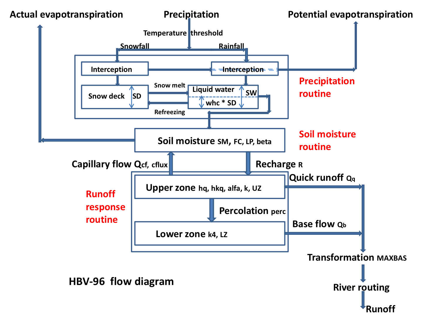
Schematic view of the relevant components of the HBV model
The figure above shows a schematic view of hydrological response simulation with the HBV-modelling concept. The land-phase of the hydrological cycle is represented by three different components: a snow routine, a soil routine and a runoff response routine. Each component is discussed separately below.
The snow routine
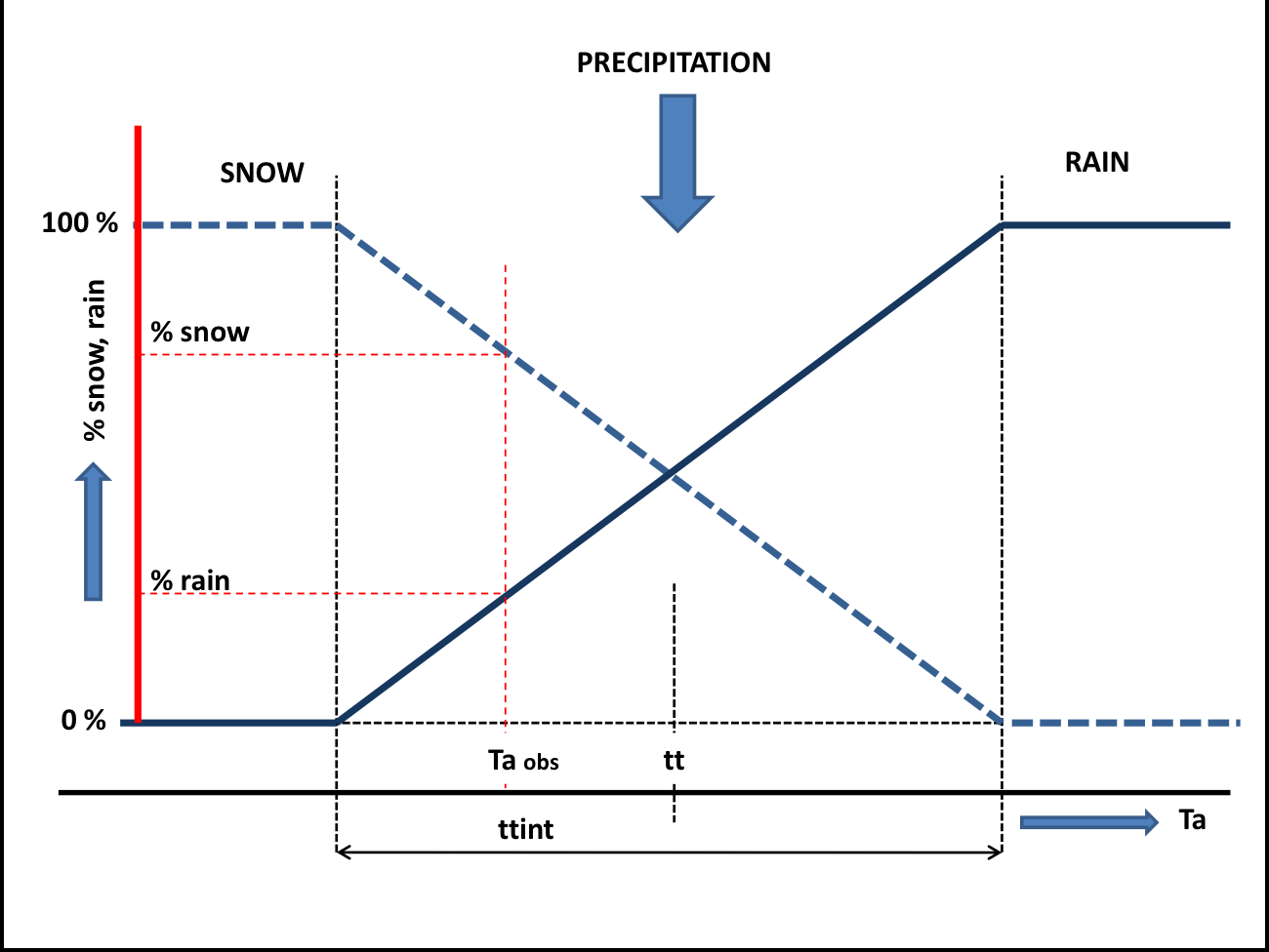
Precipitation enters the model via the snow routine. If the air temperature, \(T_{a}\), is below a user-defined threshold \(TT (\approx0^{o}C)\) precipitation occurs as snowfall, whereas it occurs as rainfall if \(T_{a}\geq TT\). A another parameter \(TTI\) defines how precipitation can occur partly as rain of snowfall (see the figure below). If precipitation occurs as snowfall, it is added to the dry snow component within the snow pack. Otherwise it ends up in the free water reservoir, which represents the liquid water content of the snow pack. Between the two components of the snow pack, interactions take place, either through snow melt (if temperatures are above a threshold \(TT\)) or through snow refreezing (if temperatures are below threshold \(TT\)). The respective rates of snow melt and refreezing are:
where \(Q_{m}\) is the rate of snow melt, \(Q_{r}\) is the rate of snow refreezing, and $cfmax$ and $cfr$ are user defined model parameters (the melting factor \(mm/(^{o}C*day)\) and the refreezing factor respectively)
Note
The FoCFMAX parameter from the original HBV version is not used. instead the CFMAX is presumed to be for the landuse per pixel. Normally for forested pixels the CFMAX is 0.6 {*} CFMAX
The air temperature, \(T_{a}\), is related to measured daily average temperatures. In the original HBV-concept, elevation differences within the catchment are represented through a distribution function (i.e. a hypsographic curve) which makes the snow module semi-distributed. In the modified version that is applied here, the temperature, \(T_{a}\), is represented in a fully distributed manner, which means for each grid cell the temperature is related to the grid elevation.
The fraction of liquid water in the snow pack (free water) is at most equal to a user defined fraction, \(WHC\), of the water equivalent of the dry snow content. If the liquid water concentration exceeds \(WHC\), either through snow melt or incoming rainfall, the surpluss water becomes available for infiltration into the soil:
where \(Q_{in}\) is the volume of water added to the soil module, \(SW\) is the free water content of the snow pack and \(SD\) is the dry snow content of the snow pack.
Schematic view of the snow routine
The snow model als has an optional (experimental) ‘mass-wasting’ routine. This transports snow downhill using the local drainage network. To use it set the variable MassWasting in the model section to 1.
# Masswasting of snow
# 5.67 = tan 80 graden
SnowFluxFrac = min(0.5,self.Slope/5.67) * min(1.0,self.DrySnow/MaxSnowPack)
MaxFlux = SnowFluxFrac * self.DrySnow
self.DrySnow = accucapacitystate(self.TopoLdd,self.DrySnow, MaxFlux)
self.FreeWater = accucapacitystate(self.TopoLdd,self.FreeWater,SnowFluxFrac * self.FreeWater )
Glaciers
Glacier processes are described in the wflow_funcs Module Glacier modelling
Potential Evaporation
The original HBV version includes both a multiplication factor for potential evaporation and a exponential reduction factor for potential evapotranspiration during rain events. The \(CEVPF\) factor is used to connect potential evapotranspiration per landuse. In the original version the \(CEVPFO\) is used and it is used for forest landuse only.
Interception
The parameters \(ICF0\) and \(ICFI\) introduce interception storage for forested and non-forested zones respectively in the original model. Within our application this is replaced by a single $ICF$ parameter assuming the parameter is set for each grid cell according to the land-use. In the original application it is not clear if interception evaporation is subtracted from the potential evaporation. In this implementation we dos subtract the interception evaporation to ensure total evaporation does not exceed potential evaporation. From this storage evaporation equal to the potential rate \(ET_{p}\) will occur as long as water is available, even if it is stored as snow. All water enters this store first, there is no concept of free throughfall (e.g. through gaps in the canopy). In the model a running water budget is kept of the interception store:
The available storage (ICF-Actual storage) is filled with the water coming from the snow routine (\(Q_{in}\))
Any surplus water now becomes the new \(Q_{in}\)
Interception evaporation is determined as the minimum of the current interception storage and the potential evaporation
The soil routine
The incoming water from the snow and interception routines, \(Q_{in}\), is available for infiltration in the soil routine. The soil layer has a limited capacity, \(F_{c}\), to hold soil water, which means if \(F_{c}\) is exceeded the abundant water cannot infiltrate and, consequently, becomes directly available for runoff.
where \(Q_{dr}\) is the abundant soil water (also referred to as direct runoff) and \(SM\) is the soil moisture content. Consequently, the net amount of water that infiltrates into the soil, \(I_{net}\), equals:
Part of the infiltrating water, \(I_{net}\), will runoff through the soil layer (seepage). This runoff volume, \(SP\), is related to the soil moisture content, \(SM\), through the following power relation:
where \(\beta\) is an empirically based parameter. Application of this equation implies that the amount of seepage water increases with increasing soil moisture content. The fraction of the infiltrating water which doesn’t runoff, \(I_{net}-SP\), is added to the available amount of soil moisture, \(SM\). The \(\beta\) parameter affects the amount of supply to the soil moisture reservoir that is transferred to the quick response reservoir. Values of \(\beta\) vary generally between 1 and 3. Larger values of \(\beta\) reduce runoff and indicate a higher absorption capacity of the soil (see Figure ref{fig:HBV-Beta}).
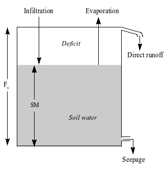
Schematic view of the soil moisture routine
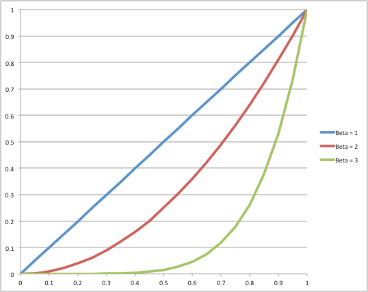
Figure showing the relation between \(SM/F_{c}\) (x-axis) and the fraction of water running off (y-axis) for three values of \(\beta\) :1, 2 and 3
A percentage of the soil moisture will evaporate. This percentage is related to the measured potential evaporation and the available amount of soil moisture:
where \(E_{a}\) is the actual evaporation, \(E_{p}\) is the potential evaporation and \(T_{m}\) (\(\leq F_{c}\)) is a user defined threshold, above which the actual evaporation equals the potential evaporation. \(T_{m}\) is defined as \(LP*F_{c}\;\) in which \(LP\) is a soil dependent evaporation factor \((LP\leq1)\).
In the original model (Berglov, 2009 XX), a correction to \(Ea\) is applied in case of interception. If \(Ea\) from the soil moisture storage plus \(Ei\) exceeds \(ETp - Ei\) (\(Ei\) = interception evaporation) then the exceeding part is multiplied by a factor (1-ered), where the parameter ered varies between 0 and 1. This correction is presently not present in the wflow_hbv model.
The runoff response routine
The volume of water which becomes available for runoff, \(S_{dr}+SP\), is transferred to the runoff response routine. In this routine the runoff delay is simulated through the use of a number of linear reservoirs.
Two linear reservoirs are defined to simulate the different runoff processes: the upper zone (generating quick runoff and interflow) and the lower zone (generating slow runoff). The available runoff water from the soil routine (i.e. direct runoff, \(S_{dr}\), and seepage, \(SP\)) in principle ends up in the lower zone, unless the percolation threshold, \(PERC\), is exceeded, in which case the redundant water ends up in the upper zone:
where \(V_{UZ}\) is the content of the upper zone, \(V_{LZ}\) is the content of the lower zone and \(\triangle\) means increase of.
Capillary flow from the upper zone to the soil moisture reservoir is modeled according to:
where \(cflux\) is the maximum capilary flux in \(mm/day\).
The Upper zone generates quick runoff \((Q_{q})\) using:
here \(K\) is the upper zone recession coefficient, and \(\alpha\) determines the amount of non-linearity. Within HBV-96, the value of \(K\) is determined from three other parameters: \(\alpha\), \(KHQ\), and \(HQ\) (mm/day). The value of \(HQ\) represents an outflow rate of the upper zone for which the recession rate is equal to \(KHQ\). if we define \(UZ_{HQ}\) to be the content of the upper zone at outflow rate \(HQ\) we can write the following equation:
If we eliminate \(UZ_{HQ}\) we obtain:
Rewriting for \(K\) results in:
Note
Note that the HBV-96 manual mentions that for a recession rate larger than 1 the timestap in the model will be adjusted.
The lower zone is a linear reservoir, which means the rate of slow runoff, \(Q_{LZ}\), which leaves this zone during one time step equals:
where \(K_{LZ}\) is the reservoir constant.
The upper zone is also a linear reservoir, but it is slightly more complicated than the lower zone because it is divided into two zones: A lower part in which interflow is generated and an upper part in which quick flow is generated (see Figure ref{fig:upper}).
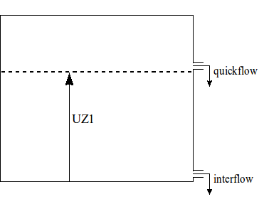
Schematic view of the Upper zone
If the total water content of the upper zone, \(V_{UZ}\), is lower than a threshold \(UZ1\), the upper zone only generates interflow. On the other hand, if \(V_{UZ}\) exceeds \(UZ1\), part of the upper zone water will runoff as quick flow:
Where \(Q_{i}\) is the amount of generated interflow in one time step, \(Q_{q}\) is the amount of generated quick flow in one time step and \(K_{i}\) and \(K_{q}\) are reservoir constants for interflow and quick flow respectively.
The total runoff rate, \(Q\), is equal to the sum of the three different runoff components:
The runoff behaviour in the runoff response routine is controlled by two threshold values \(P_{m}\) and \(UZ1\) in combination with three reservoir parameters, \(K_{LZ}\), \(K_{i}\) and \(K_{q}\). In order to represent the differences in delay times between the three runoff components, the reservoir constants have to meet the following requirement:
Subcatchment flow
Normally the the kinematic wave is continuous throughout the model. By using the the SubCatchFlowOnly entry in the model section of the ini file all flow is at the subcatchment only and no flow is transferred from one subcatchment to another. This can be handy when connecting the result of the model to a water allocation model such as Ribasim.
Example:
[model]
SubCatchFlowOnly = 1