The wflow_topoflex Model
Introduction
Topoflex applies the concept of using different model configurations for different hydrological response units (HRUs) . These HRUs can for a large part be derived from topography ([savenije]); however, additional data such as land use and geology can further optimize the selection of hydrological response units. In contrast to other models, topoflex generally uses a minimum amount of HRUs, which are defined manually, i.e. 2-5 depending on the size of and the variablity within the catchment. Nevertheless, the model code is written such that it can handle an infinte number of classes. The individual HRUs are treated as parallel model structures and only connected via the groundwater reservoir and the stream network.
The model code is written in a modular setup: different conceptualisations can be selected for each reservoir for each HRU. The code currently contains some reservoir conceptualisations (see below), but new conceptualisations can easily be added.
Examples of the application of topoflex can be found in Gharari et al. (2014), Gao et al. (2014) and Euser et al. (2015).
Figure 1 shows a possible model conceptualistion: one that used two HRUs (wetland (W) and hillslope (H), adapted from [euser])
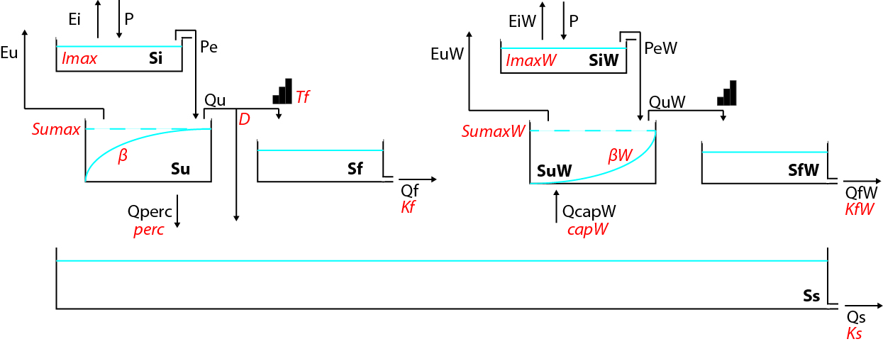
Schematic view of the relevant components of the topoflex model
Limitations
Using a set of HRUs introduces additional complexity (structural and computational) in the model. Therefore,
calibration of the model should be carried out carefully (see below for some tips and tricks that might help).
The selection and deliniation of the HRUs is a relatively subjective exercise: different data sources and
preferably some expert knowledge migth help to construct meaningful HRUs.
Spatial resolution
The model uses a grid based on the available input or required output data. The combination with the HRUs has to be done in the preparation step: for each cell the percentage of each class needs to be determined and stored in a staticmap.
The cell sizes do not have to have the same size: the size of individual cells can be stored in a staticmap, which is used to calculate the contribution of each cell to the generated discharge.
Input data
The required input data consists of timeseries of precipitation, temperature potential evaporation. In case the Jarvis equations are used to determine transpiration more input variable are required, such as humidity, radiation, wind speed and LAI.
Different HRUs
Currently there are conceptualisations for three main HRUs: wetland, hillslope and (agricultural) plateau. These conceptualisations are simply a set of reservoirs, which match the perception of different landscape elements (in western Europe). Dependent on the area or interest the HRUs can be adapted, was well as the set of reservoirs per HRU.
wetland
Wetlands are areas close to the stream, where the groundwater levels are assumed to be shallow and assumed to rise quickly during an event. The dominant runoff process in wetlands is assumed to be saturation overland flow, leading to quick and sharp responses to rainfall.
hillslope
Hillslopes are steep areas in an catchment, generally covered with forest. The dominant runoff process is assumed to be quick subsurface flow: the hillslopes mainly contribute to the discharge during the winter period.
(agricultural) plateau
Plateus are flat areas high above the stream, thus with deep ground water levels. Depending on the specific conditions, the dominant runoff processes are ground water recharge, quick subsurface flow and hortonian overland flow. The latter is especially important in agricultural areas.
Other modelling options
Routing of generated discharge
The routing of generated discharge is based on the average velocity of water through the river, which is currently set to 1 m/s. For each cell the average distance to the outlet is calculated and multiplied with the selected flow velocity to determine the delay at the outlet.
There are currently two options to apply this routing:
only calculating the delay relevant for the discharge at the outlet
calculating the delay (and thus discharge) over the stream network. This option is mainly relevant for calculations with a finer grid
Calibrating the wflow_topoflex model
Including more HRUs in the model leads to an increase in parameters. To make it still feasible to calibrate the model, a set of constraints is introduced: parameter and process constraints. These constraints are assumed relations
between parameters and fluxes of different HRUs and prevent the selection of unreaslistic parameters. The constraints are an important part of the perceptual model, but are not (yet) included in de wflow code. Below some examples of constraints are given, more examples of constraints can be found in Gharari et al. (2014), Gao et al. (2014) and Euser et al. (2015).
Parameter constraints
Parameter constraints are relations between parameters of different HRUs, for example the root zone storage capacity ( S_{u,max}), which is assumed to be larger on hillslopes than in wetlands. As in the latter groundwater levels quicky rise during a rain event, reducing the root zone storage capacity. Parameter constraints are calculated before the model runs.
Process constraints
Process constraints are comparable with parameter constraints, but focus on fluxes from different HRUs, for example the fast response from the wetlands is assumed to be larger than the fast response of the hillslopes in the summer period. As on the hillslopes generally more storage is required before a runoff generation threshold is exceeded. Process constraints are calculated after the model runs.
References
Euser, T., Hrachowitz, M., Winsemius, H. C. and Savenije, H. H. G.: The effect of forcing and landscape distribution on performance and consistency of model structures. Hydrol. Process., doi: 10.1002/hyp.10445, 2015.
Gao, H., Hrachowitz, M., Fenicia, F., Gharari, S., and Savenije, H. H. G.: Testing the realism of a topography-driven model (FLEX-Topo) in the nested catchments of the Upper Heihe, China, Hydrol. Earth Syst. Sci., 18, 1895-1915, doi:10.5194/hess-18-1895-2014, 2014.
Gharari, S., Hrachowitz, M., Fenicia, F., Gao, H., and Savenije, H. H. G.: Using expert knowledge to increase realism in environmental system models can dramatically reduce the need for calibration, Hydrol. Earth Syst. Sci., 18, 4839-4859, doi:10.5194/hess-18-4839-2014, 2014.
Savenije, H. H. G.: HESS Opinions “Topography driven conceptual modelling (FLEX-Topo)”, Hydrol. Earth Syst. Sci., 14, 2681-2692, doi:10.5194/hess-14-2681-2010, 2010.
example ini file
The .ini file below shows the available options
[framework]
outputformat = 1

# Model parameters and settings
[model]
## The settings below define the way input data is handeled
# ScalarInput: 0 = input from mapstacks (.map); 1 = input from timeseries (.tss)
ScalarInput=1
# InputSeries can be used if multiple sets of input series are available, TE: maybe better to remove this option?
InputSeries=1
# InterpolationMethod: inv = inverse distance,  pol = Thiessen polygons, this option is not relevant if the number of cells is equal to the number of meteo gauges
InterpolationMethod=inv

##  Remaining model settings
# L_IR(UR(FR)) indicates with reservoirs are treated lumped with regard to moisture states. 0 = distributed; 1 = lumped. IR = interception reservoir; UR = unsaturated zone reservoir; FR = fast runoff reservoir
L_IRURFR = 0
L_URFR = 0
L_FR = 0
# maxTransitTime is the travel time (same time resolution as model calculations) through the stream of the most upstream point, rounded up
maxTransitTime = 9
# DistForcing is the number of used rainfall gauges
DistForcing = 3
# maxGaugeId is the id of the raingauge with the highest id-number, this setting has to do with writing the output data for the correct stations
maxGaugeId = 10
# timestepsecs is the number of seconds per time step
timestepsecs = 3600

## the settings below deal with the selection of classes and conceptualisations of reservoirs
## classes indicates the number of classes, the specific characters are not important (will be used for writing output??), but the number of sets of characters is important
classes = ['W','H']

## selection of reservoir configuration - 'None' means reservoir should not be modelled for this class
selectSi = interception_overflow2, interception_overflow2
selectSu= unsatZone_LP_beta, unsatZone_LP_beta
selectSus=None,None
selectSf=fastRunoff_lag2, fastRunoff_lag2
selectSr=None,None

## selection of Ss (lumped over entire catchment, so only one!)
# selectSs = <some other reservoir than groundWaterCombined3>

## wflow maps with percentages, the numbers correspond to the indices of the characters in classes.
wflow_percent_0 = staticmaps/wflow_percentW4.map
wflow_percent_1 = staticmaps/wflow_percentHPPPA4.map

##constant model parameters - some are catchment dependent
Ks = 0.0004
lamda = 2.45e6
Cp = 1.01e-3
rhoA = 1.29
rhoW = 1000
gamma = 0.066
JC_Topt = 301

#parameters for fluxes and storages
sumax = [140, 300]
beta = [0.1, 0.1]
D = [0, 0.10]
Kf = [0.1, 0.006]
Tf = [1, 3]
imax = [1.2, 2]
perc = [0, 0.000]
cap = [0.09, 0]
LP = [0.5, 0.8]
Ce = [1, 1]

#parameters for Jarvis stressfunctions
JC_D05 = [1.5,1.5]
JC_cd1 = [3,3]
JC_cd2 = [0.1,0.1]
JC_cr = [100,100]
JC_cuz = [0.07,0.07]
SuFC = [0.98,0.98]
SuWP = [0.1,0.1]
JC_rstmin = [150,250]

[layout]
# if set to zero the cell-size is given in lat/long (the default)
sizeinmetres = 0

[outputmaps]
#self.Si_diff=sidiff
#self.Pe=pe
#self.Ei=Ei

# List all timeseries in tss format to save in this section. Timeseries are
# produced per subcatchment.

[outputtss_0]
samplemap=staticmaps/wflow_mgauges.map
#states
self.Si[0]=SiW.tss
self.Si[1]=SiH.tss
self.Sf[1]=SfH.tss
self.Sf[0]=SfW.tss
self.Su[1]=SuH.tss
self.Su[0]=SuW.tss
#fluxen
self.Precipitation=Prec.tss
self.Qu_[0]=QuW.tss
self.Qu_[1]=QuH.tss
self.Ei_[0]=EiW.tss
self.Ei_[1]=EiH.tss
self.Eu_[0]=EuW.tss
self.Eu_[1]=EuH.tss
self.Pe_[0]=peW.tss
self.Pe_[1]=peH.tss
self.Perc_[1]=PercH.tss
self.Cap_[0]=CapW.tss
self.Qf_[1] = QfH.tss
self.Qf_[0] = QfW.tss
self.Qfcub = Qfcub.tss
self.Qtlag = Qtlag.tss

[outputtss_1]
samplemap = staticmaps/wflow_gauges.map
#states
self.Ss = Ss.tss
#fluxen
self.Qs = Qs.tss
self.QLagTot = runLag.tss
self.WBtot = WB.tss

[modelparameters]
# Format:
# name=stack,type,default,verbose[lookupmap_1],[lookupmap_2],lookupmap_n]
# example:
# RootingDepth=monthlyclim/ROOT,monthyclim,100,1

# - name - Name of the parameter (internal variable)
# - stack - Name of the mapstack (representation on disk or in mem) relative to case
# - type - Type of parameter (default = static)
# - default - Default value if map/tbl is not present
# - set to 1 to be verbose if a map is missing
# - lookupmap - maps to be used in the lookuptable in the case the type is statictbl

#Possible types are::
# - staticmap: Read at startup from map
# - statictbl: Read at startup from tbl
# - tbl: Read each timestep from tbl and at startup
# - timeseries: read map for each timestep
# - monthlyclim: read a map corresponding to the current month (12 maps in total)
# - dailyclim: read a map corresponding to the current day of the year
# - hourlyclim: read a map corresponding to the current hour of the day (24 in total) (not implemented yet)
# - tss: read a tss file and link to lookupmap (only one allowed) a map using timeinputscalar
Precipitation=intss/1_P.tss,tss,0.0,1,staticmaps/wflow_mgauges.map
Temperature=intss/1_T.tss,tss,10.5,1,staticmaps/wflow_mgauges.map
PotEvaporation=intss/1_PET.tss,tss,0.0,1,staticmaps/wflow_mgauges.map
An example ini file be found here.