The wflow_lintul Model
Introduction
Wflow_lintul, a raster-based crop growth model for rice, is based on LINTUL3, a point-based model for simulating nitrogen-limited rice growth (Shibu et al., 2010). LINTUL3 was parameterized and calibrated for rice by Shibu et al. (2010), based on experimental data from Southeast Asia (Drenth et al., 1994) and drawing on the more complex rice model ORYZA2000 (Bouman et al., 2001) and the preceding versions LINTUL1 (Spitters, 1990) and LINTUL2 (Spitters and Schapendonk, 1990). In contrast to LINTUL3, wflow_lintul is primarily intended for simulation of rice production under water-limited conditions, rather than under nitrogen-limited conditions. To that end, it was designed to function in close cooperation with the spatial hydrological model wflow_sbm, which operates on a watershed-scale.
The LINTUL (Light Interception and Utilization) models were the first deviation from the more complex, photosynthesis-based models of the “De Wit school” of crop modelling, also called the “Wageningen school” (Bouman et al., 1996). In the LINTUL models, total dry matter production is calculated in a comparatively simple way, using the Monteith approach (Monteith, 1969; 1990). In this approach, crop growth is calculated as the product of interception of (solar) radiation by the canopy and a fixed light-use efficiency (LUE; Russell et al., 1989). This way of estimating (daily) biomass production in the LINTUL models is reflected in the equation below and may be considered the core of the wflow_lintul model:
GTOTAL = self.LUE * PARINT * TRANRF
with GTOTAL the overall daily growth rate of the crop (g m\(^{-2}\) d\(^{-1}\)), self.LUE a constant light use efficiency (g MJ\(^{-1}\)), PARINT the daily intercepted photosynthetically active radiation (MJ m\(^{-2}\) d\(^{-1}\)), TRANRF (-) the ‘transpiration reduction factor’, i.e. the reducing impact of water shortage on biomass production.
For regional studies, LINTUL-type models have the advantage that data input requirements are drastically reduced and model parameterization is facilitated (Bouman et al., 1996). LINTUL was first developed for potential crop growth (i.e. perfect growing conditions without any water or nutrient shortages and in absence of pests, diseases and adverse soil conditions) as “LINTUL1” (Spitters, 1990). Later, it was extended to simulate water-limited conditions (“LINTUL2”; Spitters and Schapendonk, 1990) and nitrogen-limited conditions (“LINTUL3”; Shibu et al., 2010). Under water-limited conditions, all growth factors except water are assumed non-limiting, i.e. ample nutrient availability, a pest-, disease- and weed-free environment and no adverse soil conditions. Under nitrogen-limited conditions, only nitrogen availability may limit crop growth. LINTUL has been successfully applied to different crops such as potato (Spitters and Schapendonk, 1990), grassland (LINGRA) (Schapendonk et al., 1998), maize (Farré et al., 2000), oilseed rape (Habekotté, 1997) and rice (Shibu et al., 2010), in potential, water-limited or nitrogen-limited situations.
Differences between wflow_lintul and LINTUL3/other LINTUL versions
Potential and water-limited simulations: Wflow_lintul presently (spring 2018) simulates potential and water-limited crop growth (the latter in conjunction with wflow_sbm). First preparations to add simulation of nitrogen-limited rice growth (LINTUL3) have been made in the present version of the model.
Water balance outsourced to wflow_sbm: The simple water balance, based on Stroosnijder (1982) and Penning de Vries et al. (1989), which was present in LINTUL2 and LINTUL3, is no longer present in wflow_lintul. All water balance-related simulation tasks are outsourced to the wflow_sbm model. On the other hand, several crop growth related tasks in the hydrology model wflow_sbm, such as the simulation of LAI (leaf area index) are now outsourced to wflow_lintul. In the wflow framework, wflow_lintul and wflow_sbm communicate with each other via the Basic Model Interface (BMI) implementation for wflow (wflow_bmi).
Written in PCRaster Python: Whereas the original LINTUL1, LINTUL2 and LINTUL3 models were implemented in the Fortran Simulation Translator (FST) software (Rappoldt and Van Kraalingen, 1996), wflow_lintul is written in PCRaster Python and fully integrated into the wflow hydrologic modelling framework.
Written in PCRaster Python: Integration of wflow_lintul in the wflow framework means that all timer and input-output related tasks for the model are handled by that framework. The original LINTUL1, LINTUL2 and LINTUL3 models were implemented in the Fortran Simulation Translator (FST) software (Rappoldt and Van Kraalingen, 1996). In FST, timer and input-output related tasks were handled by the TTUTIL library (a collection UTILities originating from the former “Theoretische Teeltkunde” research group of Wageningen University and Research; Rappoldt and Van Kraalingen, 1996).
Raster based: In contrast to LINTUL1, 2 and 3, most input and output variables in wflow_lintul are represented by maps or arrays, instead of single values (unless a base-map with a dimension of only one grid cell is specified). Each value in such a map or array represents a grid cell on the map of the study area/catchment; wflow-lintul simulates crop growth for all grid cells simultaneously and can therefore be characterized as a grid-based model. The original LINTUL1, LINTUL2 and LINTUL3 models, in contrast, were point-based and only able to simulate crop growth for one grid cell at a time.
Runs for multiple consecutive seasons or years: As opposed to the original LINTUL models, which run for one season/year at a time, wflow_lintul can continuously run over multiple consecutive cropping cycles and years. At the end of each cropping season, the crop is then harvested automatically, meaning that all variables are reset. At the beginning of each new cropping season, crop growth is automatically re-initiated.
Advanced and remotely sensed run control: Wflow_lintul offers various novel options for controlling the onset and termination of crop growth:
1. Crop growth can be initiated automatically, on a pixel-by-pixel basis, based on remotely sensed data. To that end, satellite imagery needs to be processed in such a way that for each pixel/grid cell, a Boolean value indicates whether there is (rice) crop growth, predominantly (value = 1), or not (value = 0). The model starts/terminates crop growth if changes 0->1 or vice versa occur.
2. Crop growth can be (automatically) initiated on a pixel-by-pixel basis if a pre-specified minimum amount of rainfall requirement has accumulated – this amount may be considered necessary for land preparation (soil puddling). In the implementation for central Java, this threshold is normally set at 200 mm rainfall from November 1 on (approximate start of the rainy season), based on Naylor et al. (2007).
3. Similar to the original point-based LINTUL models, the user can enter a single fixed start date and/or a single fixed end date; these dates will then be applied across all grid cells of the simulated catchment area simultaneously. To simulate growth of transplanted rice, which has already emerged and grown for some time in the nursery before being planted out in the main field, a default initial development stage is specified in the model, together with initial weights of leaves, stems and roots.
Run options
Running wflow_lintul standalone (potential production)
For runs, i.e. without linking to the hydrology model wflow_sbm, the “WATERLIMITED” option in the wflow_lintul.ini should be set to “False”. Water limited simulation presently requires the presence of a water balance/hydrology model (i.e. wflow_sbm).
Running wflow_lintul in conjunction with wflow_sbm
For running wflow_lintul in conjunction with the hydrological model wflow_sbm, which takes care of all water-balance related tasks and which is what the model is really intended for, a Python BMI runner module, exchanging data between wflow_sbm and wflow_lintul, needs to be run.
An example of a coupled wflow_sbm and wflow_lintul model is available in \wflow\examples\wflow_brantas_sbm_lintul
To run the coupled models:
activate wflow
python bmi2runner.py bmi2runner.ini
Settings for wflow_lintul
List of run control parameters
Wflow_lintul model runs can be configured by editing the values of a number of parameters in the [model] section of the wflow_lintul.ini file. Wflow_lintul reads the values from wflow_lintul.ini with its parameters function; if a certain parameter or value is not found in wflow_lintul.ini, a default value (provided for each individual parameter in the parameters function) is returned. The following nine variables in wflow_lintul.ini have a run control function:
[model]
CropStartDOY = 0
HarvestDAP = 90
WATERLIMITED = True
AutoStartStop = True
RainSumStart_Month = 11
RainSumStart_Day = 1
RainSumReq = 200
Pause = 13
Sim3rdSeason = True
For each of these control variables, additional explanation is explained below:
CropStartDOY (integer) - needs to be set to 0 if set from outside. Sets the Julian Day Of the Year (DOY) on which crop growth is initiated – for all grid cells simultaneously. If set to 0, crop growth is initiated automatically for each grid cell individually, based on a certain minimum accumulated rainfall quantity (AutoStartStop is set to True) or based on remote sensing information (if AutoStartStop is set to False; see also Run Control variable 4, AutoStartStop).
HarvestDAP (integer): sets the number of Days After Planting (DAP) on which crop growth is terminated and all crop-related states are reset to 0 – for all grid cells simultaneously. It is advisable to set HarvestDAP = 0, so that crop growth is terminated when the crop is physiologically mature, on a pixel by pixel basis. For rice in Indonesia, this is generally the case after 80-110 DAP. If a positive HarvestDAP value is set and the crop is not yet physiologically mature after the specified number of days, the crop will be harvested immaturely (simultaneously in all pixels). If the crop had already reached physiological maturity before the specified number of DAP, the last simulated values of the state variable (final rice yield, LAI, etc.) will be maintained until the specified number of DAP is reached and then be reset to 0 in all pixels simultaneously.
WATERLIMITED (Boolean): if WATERLIMITED = False, potential crop growth will be simulated, i.e. crop growth without any water limitation (definition: see Introduction). With this option, wflow_lintul can also be run standalone (i.e. without coupling to the hydrological model wflow_sbm). If WATERLIMITED = True (default), evapotranspiration and soil water status will be simulated by the wflow_sbm model and crop growth will be reduced in case of less-than-perfect water supply (water-limited production).
AutoStartStop (Boolean): if set to True, rice crop growth in the rainy season will be initiated automatically for each grid cell (unless CropStartDOY is set > 0), based on the cumulative amount of precipitation that falls in that grid cell from November 1 on (this date can be changed by adjusting RainSumStart_Month and RainSumStart_Day in wflow_lintul.ini, see Section 4, run control variables 5 and 6). If a pre-specified threshold value (RainReqStartSeason_1, default value 200 mm; see Section 4, run control variable 7) is reached, rice crop growth will be initiated.
The second (dry season) crop will be initiated at a specified number of days after termination of the first (wet season) crop. This period allows for harvesting operations and preparation of the new field to take place and can be changed by modifying the value of the variable “Pause”. Similarly, the third (dry season) crop will be initiated at the specified number of days after termination of the second (dry season) crop.
Crop growth during the second season will, similar to the first season, be terminated when the accumulated temperature sum (model internal variable self. TSUM) reaches TTSUM, or at the specified number of days after crop establishment (HarvestDAP) - whichever occurs first.
For all three simulated seasons, crop growth in a certain grid cell will cease - and a final rice yield estimate will be obtained - when the accumulated temperature sum (model internal variable self.TSUM) reaches TTSUM, i.e. the total temperature sum required to reach crop maturity. However, if HarvestDAP is set > 0, crop growth will cease after the specified number of DAP is reached, or when TTSUM is reached – whichever occurs first.
RainSumStart_Month (integer): the month of the year from which the accumulated amount of precipitation (required for initiating the first, rainy, season) is starting to be calculated. Crop simulation starts if the amount (in mm) meets RainReqStartSeason_1.
RainSumStart_Day (integer): the day of the planting month (RainSumStart_Month; parameter 5., above) from which the accumulated amount of precipitation (required for initiating the first, rainy, season) is calculated. Crop simulation starts if the amount (in mm) meets RainReqStartSeason_1.
RainSumReq (real, mm): the accumulated amount of precipitation (in mm) that is required for establishment of the irrigated rice crop at the start of the first (rainy) season.
Pause (integer, days): the number of days between the first (rainy) and second (dry) season and between the second and the third season (if applicable); this period is required for harvesting, land preparation and planting of the second and/or third crop.
Sim3rdSeason (Boolean): if set to True, a third rice crop will be simulated in each simulated year. In case it has not matured on the date specified by Run Control variables 5 and 6, the third crop will be terminated on that date, assuming that farmers will prioritize the first (main) rainy season crop and that in such situations (cooler places), planting 3 rice crops per year is probably not worthwhile.
List of model parameters
[model]
LAT = 3.16
LUE = 2.47
TSUMI = 362
K = 0.6
SLAC = 0.02
TSUMAN = 1420
TSUMMT = 580.
TBASE = 8.
RGRL = 0.009
WLVGI = 0.86
WSTI = 0.71
WRTLI = 1.58
WSOI = 0.00
DVSDR = 0.8
RDRRT = 0.03
RDRSHM = 0.03
LAICR = 4.0
ROOTDM_mm = 1000.
RRDMAX_mm = 10.
ROOTDI_mm = 50.
RDRTB = [0.0,0.0, 0.6,0.00, 1.0,.015, 1.6,0.025, 2.1,0.05, "RDRTB"]
PHOTTB = [0.0,0.0, 8.0,0.0, 10.0,1.0, 12.0,1.0, 13.0,0.8, 14.0,0.6, 18.,0.0, "PHOTTB"]
SLACF = [0.0,1.72, 0.21,1.72, 0.24,1.72, 0.33,1.32, 0.7,1.20,1.01,1.00, 2.0,0.75, 2.1,0.75, "SLACF"]
FRTTB = [0.0,0.300, 0.48,0.30, 0.62,0.12, 0.69,0.11, 0.84,0.1,.92,0.10, 1.00,0.08, 1.38,0.00, 2.11,0.0, "FRTTB"]
FLVTB = [0.0,0.315, 0.48,0.35, 0.62,0.44, 0.69,0.463, 0.84,0.463, 0.92,0.45, 1.00,0.00, 1.38,0.00, 2.10,0.0, "FLVTB"]
FSTTB = [0.0,0.385, 0.48,0.35, 0.62,0.44, 0.69,0.427, 0.84,0.427, 0.92,0.27, 1.00,0.00, 1.38,0.00, 2.10,0.0, "FSTTB"]
FSOTB = [0.0,0.00, 0.48,0.00, 0.62,0.00, 0.69,0.00, 0.84,0.00, 0.92,0.18, 1.00,0.92, 1.38,1.00, 2.10,1.00, "FSOTB"]
For each of the above parameters, additional explanation is explained below:
LAT (real, degrees): the geographic latitude, required for calculation of the correct astronomic day length for each day of the simulation; day length may influence crop-physiological processes such as the allocation of carbohydrates, the initialization of flowering, etc. It assumed that day length is identical throughout the simulated catchment area; in very large catchments it might, theoretically, be preferable to calculate the day length for each individual grid cell. Actual day length calculations are based on the FORTRAN subroutine SASTRO (Van Kraalingen, 1995) which is, in turn, based on Goudriaan and van Laar (1994, around p.30).
LUE (real, g biomass MJ:math:`^{-1}` of intercepted solar radiation): the light use efficiency of the crop or variety that is simulated. For rice, the default value is 3.0 (Shibu et al., 2010). To account for different varieties, management imperfections or adverse conditions, a different value may be obtained by local calibration with observed rice yields, preferably of well-managed experiments that approach potential or water limited growing conditions, i.e. in absence of nutrient shortages, toxic elements or pests and diseases. The potential yield level is determined by the growth-defining factors, i.e. incoming solar radiation, temperature and characteristics of the crop when the crop is optimally supplied with water and nutrients and is completely protected against growth-reducing factors. Water-limited and nutrient-limited yield levels are lower than the potential, due to a suboptimal supply of water and/or nutrients, respectively. The actual production level is determined by actual supplies of water and nutrients, and by the degree that the crop is protected against growth-reducing factors or escapes their effects (Van Ittersum and Rabbinge, 1997). Alternatively, if the LUE of wflow_lintul is calibrated against actual farm yields, the model may be used to predict actual crop yields, instead of water-limited or potential crop yields, taking into the account the average occurrence nutrient shortages, toxic elements or pests and diseases in the relevant region and over the relevant period of time.
TSUMI (real, degree days): the initial temperature sum (at the moment of transplanting, only relevant for transplanted rice).
K (real, dimensionless): the light extinction coefficient (for rice leaves). Light interception in LINTUL increases with LAI according to a negative exponential pattern, characterized by a crop-specific light extinction coefficient (K, m\(^{2}\) (ground) m\(^{-2}\) (leaf)): an implementation of Lambert-Beer’s law.
SLAC (real, m:math:`^{2}` (leaf) g:math:`^{-1}` (leaf)): Specific Leaf Area Constant, introduced by Shibu et al. (2010). SLAC is multiplied by SLACF, a Leaf area correction function as a function of development stage to obtain SLA, the specific leaf area (real, m\(^{2}\) (leaf) g\(^{-1}\) (leaf)).
TSUMAN (real, degree days): the temperature sum required for the crop to reach anthesis.
TSUMMT (real, degree days): the temperature sum required for the crop to develop from anthesis to maturity (rice ready for harvest).
TBASE (real, degrees centigrade): since many growth processes are temperature dependent above a certain threshold temperature, only temperatures above a certain minimum temperature (TBASE, real, degrees centigrade) lead to increase in temperature sum/crop phenological development. For rice, TBASE is 8 °C (Shibu et al., 2010) hence below that temperature, no crop development takes place.
RGRL (real, dimensionless): the relative (daily) growth rate of leaf area during the exponential growth phase, expressed per degree-day.
WLVGI, WSTI, WRTLI, WSOI: Initial weight (at transplanting time) of green leaves, stems, roots and storage organs (i.e. rice grains), respectively, in g DM m−2.
DVSDR (real, dimensionless): value of the Crop Development Stage, DVS) above which the death of leaves and roots sets in.
RDRRT (real, dimensionless): relative (daily) death rate of roots.
RDRSHM (real, dimensionless): maximum relative (daily) death rate of leaves due to shading.
LAICR (real, dimensionless): value of the crop Leaf Area Index (LAI) above which mutual shading of leaves occurs which may in turn influence the death rate of leaves.
ROOTDM_mm (real, mm): maximum rooting depth for a rice crop.
RRDMAX_mm (real, mm d:math:`^{-1}`): maximum daily increase in rooting depth (m) for a rice crop.
ROOTDI_mm (real, mm): initial rooting depth (after transplanting).
RDRTB (real, dimensionless): interpolation table defining the relative (daily) death rate of leaves (RDRTMP) as a function of Developmental Stage. Adopted by Shibu et al. (2010) from Bouman et al. (2001).
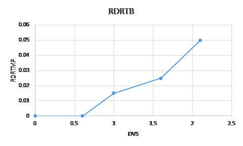
The RDRTB parameter (list) defines the relative (daily) death rate of leaves (RDRTMP) as a function of crop Developmental Stage (DVS)
PHOTTB (real, dimensionless): interpolation table defining the modifying effect of photoperiodicity on the phenological development rate (from LINTUL3/Shibu et al. 2010 - original source unclear) as a function of daylength (DAYL, hours).
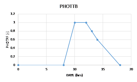
The PHOTTB parameter (table) defines the modifying effect of photoperiodicity on the phenological development rate as a function of day length (DAYL)
SLACF (real, dimensionless): interpolation table defining the leaf area correction factor (SLACF) as a function of development stage (DVS; Drenth et al., 1994). The Specific Leaf Area Constant (SLAC) is multiplied with a correction factor to obtain the specific leaf area (SLA); this correction factor, in turn, is obtained by linear interpolation in the SLACF table (Figure 3), using the relevant value of DVS as independent variable.
SLA = self.SLAC * self.SLACF.lookup_linear(self.DVS)where self.SLACF.lookup_linear(self.DVS) results in the relevant value of the correction factor by linear interpolation based on DVS.
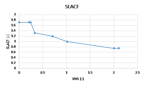
The SLACF interpolation table defines the leaf area correction factor (SLACF) as a function of development stage (DVS)
FRTTB (real, dimensionless): interpolation table defining the fraction of daily dry matter production allocated to root growth (FRTWET), in absence of water shortage, as a function of development stage (DVS). FRTWET is obtained by linear interpolation in FRTTB, with DVS as the independent variable.
FRTWET = self.FRTTB.lookup_linear(self.DVS)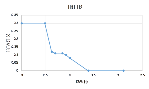
The FRTTB interpolation table defines the fraction of daily dry matter production allocated to root growth (FRTWET) in absence of water shortage as a function of the crop development stage (DVS).
FLVTB (real, dimensionless): interpolation table defining the fraction of daily dry matter production allocated to growth of leaves (FLVT), in absence of water shortage, as a function of development stage (DVS). FLVT is obtained by linear interpolation in FLVTB, with DVS as the independent variable:
FLVT = self.FLVTB.lookup_linear(self.DVS)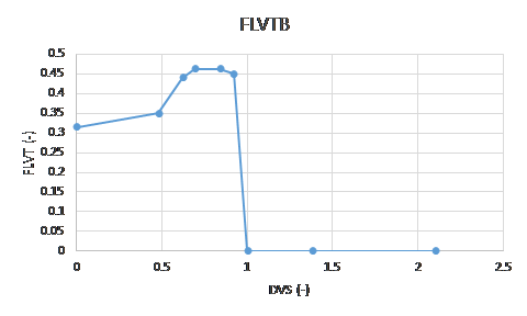
The FLVTB interpolation table defines the fraction of daily dry matter production allocated to growth of leaves (FLVT) in absence of water shortage, as a function of development stage.
FSTTB (real, dimensionless): interpolation table defining the fraction of daily dry matter production allocated to growth of stems (FSTT), in absence of water shortage, as a function of development stage (DVS). FSTT is obtained by linear interpolation in FSTTB, with DVS as the independent variable:
FSTT = self.FSTTB.lookup_linear(self.DVS)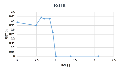
The FSTTB interpolation table defines the fraction of daily dry matter production allocated to growth of stems (FSTT) in absence of water shortage, as a function of the crop development stage (DVS).
FSOTB (real, dimensionless): interpolation table defining the fraction of daily dry matter production allocated to growth of stems (FSOT), in absence of water shortage, as a function of development stage (DVS; Figure 7). FSOT is obtained by linear interpolation in FSOTB, with DVS as the independent variable:
FSOT = self.FSOTB.lookup_linear(self.DVS)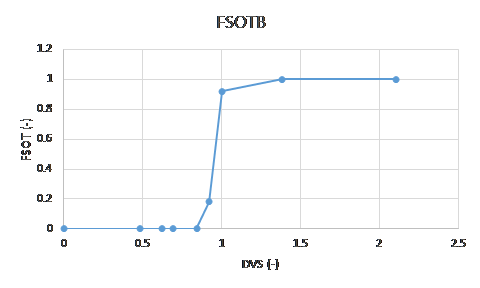
The FSOTB interpolation table defines the fraction of daily dry matter production allocated to growth of stems (FSOT), in absence of water shortage, as a function of the crop development stage (DVS).
Model forcing data
In terms of meteorological data, wflow_lintul requires daily values of:
Solar radiation (IRRAD; kJ m\(^{-2}\) d\(^{-1}\))
Average temperature (T; °C)
Precipitation (RAIN, mm)
For water-limited simulations, LINTUL-type models normally also require data of vapour pressure and wind speed for calculating evapotranspiration. However, in the case of wflow_lintul, actual (rice) crop transpiration (Transpiration; mm d\(^{-1}\)) and potential (rice) crop transpiration (PotTrans; mm d\(^{-1}\)) under water-limited crop growth are calculated by the wflow_sbm hydrologic model which then supplies these variables to wflow_lintul via the BMI. They are then used for calculating TRANRF, a factor that describes the reducing effect of water shortage on biomass production.
Wflow_sbm, in turn, requires potential evaporation as a forcing variable. Similarly, water content in the rooted zone (self.WA) is simulated by wflow_sbm and then transferred to wflow_lintul via the BMI.
In turn, for wflow_sbm being able to perform these calculations, wflow_lintul supplies it with daily values of LAI (m\(^{2}\) leaf m\(^{-2}\) ground) and rooting depth to wflow_sbm, again via the BMI.
Description of core wflow_lintul model code
Phenology
Phenological development of crops is generally closely related to thermal time, i.e. the accumulated number of degree-days after emergence. Instead of simply adding up degree-days, a daily effective temperature (DTEFF, °C d) is used in wflow_lintul however, since many growth processes are only temperature dependent, or only occur, above a certain threshold temperature. DTEFF is calculated according to:
DTEFF = ifthenelse(Warm_Enough, DegreeDay, 0.)
with DTEFF the daily effective temperature (°C d), Warm_Enough a Boolean variable that equals True when the daily average temperature T is larger than or equal to TBASE, the base temperature for a rice crop (°C). DegreeDay is the daily average temperature reduced with TBASE:
DegreeDay = self.T - self.TBASE
Thus, if T is great than TBASE, DTEFF is set equal to DegreeDay; in all other cases it is set to 0. In addition, before DTEFF is added to TSUM (state variable), it is corrected for the potentially modifying effect of day length (photoperiodicity) resulting in the daily increase in temperature sum RTSUMP (°C d), according to:
RTSUMP = DTEFF * PHOTPF
where RTSUMP is the daily increase in temperature sum (°C d), modified by the influence of photoperiod DTEFF the daily effective temperature (°C d), PHOTPF is a correction factor that accounts for the modifying influence of day length on crop development via DTEFF; it is defined as a function of day length (DAYL). PHOTPF is less than 1 if day length (DAYL, hours) is shorter than 10 hours or longer than 12 hours. Day lengths between 10-12 hours have no modifying influence on DTEFF; phenological development is thus slowed down in such cases. DAYL in wflow_lintul is calculated by the function astro_py , a Python implementation of a FORTRAN subroutine from the Wageningen school of models, dating back to Spitters et al. (1989) and likely even further.
Calculation of TSUM (model state variable) by accumulating daily values of RTSUMP is then done according to:
self.TSUM = (self.TSUM + ifthenelse(CropStartNow, scalar(self.TSUMI), 0.) +
ifthenelse(EMERG, RTSUMP, 0.)) * ifthenelse(CropHarvNow, scalar(0.), 1.)
with self.TSUM the temperature sum (a crop state variable, °C d), CropStartNow: a Boolean variable that equals True on the moment of crop growth initiation TSUMI (real, degree days): the initial temperature sum (at the moment of transplanting, only relevant for transplanted rice), EMERG is a Boolean variable that indicates whether crop growth occurs; it equals True, when three conditions are met:
crop growth has been initiated
the water content of the soil is larger than the water content at permanent wilting point
LAI is greater than 0.
CropHarvNow a Boolean variable that only equals True on the day that the crop is being harvested
Thus, the state of TSUM of the previous day is increased (on the current day) with the initial temperature at the moment of transplanting/initiation of crop growth, and increased with the daily increase in (effective) temperature during the subsequent period of crop growth. At the moment of harvest (when :math:CropHarvNow = True), the third ifthenelse statement will return a zero value, hence multiplying TSUM with zero (effectively resetting it). Regarding the influence of TSUM on rice crop development two crop-specific parameters are of paramount importance, since assimilates are partitioned differently over the different plant organs before flowering (vegetative growth) than after flowering (generative growth):
TSUMAN, the value of TSUM at which crop anthesis is initiated (1420 °C d for rice variety IR72)
TSUMMT, the change in TSUM required for the crop to develop from anthesis to maturity (hence ripened rice grain can be harvested) - 580 °C d for rice variety IR72.
In LINTUL1 and LINTUL2, TSUM controls all processes that are influenced by crop phenological development. However, Shibu et al. (2010) derived important parts of LINTUL3 (for rice) from ORYZA2000 (Bouman et al., 2001). In ORYZA2000, most processes are steered by a variable called DVS (development stage; -). The development stage of a plant defines its physiological age and is characterized by the formation of the various organs and their appearance. The key development stages for rice distinguished in ORYZA2000 are emergence (DVS = 0), panicle initiation (DVS = 0.65), flowering (DVS = 1), and physiological maturity (DVS = 2; Bouman et al., 2001). Shibu et al. incorporated DVS into LINTUL which is why some processes are controlled directly by TSUM and others are controlled by its derived variable DVS – a situation that seems to offer scope for future improvement. In wflow_lintul, the key development stages emergence, flowering and physiological maturity coincide with TSUM = 0, TSUM = 1420 (flowering) and TSUM = 2000 (140 + 580; crop maturity), respectively. Panicle initiation (at DVS = 0.65) is not a significant event in wflow_lintul. DVS is calculated from :math:TSUM according to the following three equations:
DVS_veg  = self.TSUM / self.TSUMAN * ifthenelse(CropHarvNow, scalar(0.), 1.)

DVS_gen  = (1. + (self.TSUM - self.TSUMAN) / self.TSUMMT) * ifthenelse(CropHarvNow, scalar(0.), 1.)

self.DVS  = ifthenelse(Vegetative, DVS_veg, 0.) + ifthenelse(Generative, DVS_gen, 0.)
where: DVS_veg: DVS during the vegetative crop stage, CropHarvNow a Boolean variable that equals True when the crop is mature or has reached a fixed pre-defined harvest date. DVS_veg: DVS during the generative crop stage, TSUMAN, the value of TSUM at which crop anthesis is initiated (1420 °C d for rice variety IR72) TSUMMT, the change in TSUM required for the crop to develop from anthesis to maturity (hence ripened rice grain can be harvested) - 580 °C d for rice variety IR72. DVS, the crop (phenological) development stage.
Hence, DVS is calculated as the sum of DVS_veg and DVS_gen; it equals 1 (flowering) if TSUM reaches TSUMAN and equals 2 (maturity) if TSUM reaches the sum TSUMAN + TSUMMT. DVS_veg and DVS_gen are both reset (multiplied with zero) when the crop is harvested.
Photosynthesis and crop growth
As outlined in the Introduction, overall assimilate production rate in wflow_lintul is calculated as the product of the Photosynthetically Active (solar) Radiation (PAR) that is intercepted by the crop canopy and a fixed Light-Use Efficiency (LUE; Russell et al., 1989). This way of estimating (daily) biomass production in the LINTUL models is reflected as follows and may be considered the core of the wflow_lintul model:
GTOTAL = self.LUE * PARINT * TRANRF
with GTOTAL the overall daily growth rate of the crop (g m\(^{-2}\) d\(^{-1}\)), self.LUE a constant light use efficiency (g MJ\(^{-1}\)), PARINT the daily intercepted photosynthetically active radiation (MJ m\(^{-2}\) d\(^{-1}\)), TRANRF (-) the ‘transpiration reduction factor’, i.e. the reducing impact of water shortage on biomass production.
The daily intercepted PAR (PARINT,MJ m\(^{-2}\) d\(^{-1}\)), is calculated as:
PARINT = ifthenelse(Not_Finished, 0.5 * self.IRRAD * 0.001 * (1. - exp(-self.K * self.LAI)), 0.)
with: Not_Finished a Boolean variable that indicates whether the crop is still growing and developing (True) or not (False). 0.5 a factor to account for the fraction of photosynthetically active radiation in the incident solar radiation. About 50% (in terms of energy) of the frequency spectrum of incident solar radiation can be used for photosynthesis by green plants. IRRAD: incident solar radiation (m\(^{-2}\) d\(^{-1}\)) as measured by e.g. a weather station. K a crop and variety-specific light extinction coefficient (-) and LAI the leaf area index (m\(^{2}\) leaf m\(^{-2}\) ground).
Calculation of growth rates
The overall daily growth of the crop (GTOTAL, g m\(^{−2}\) d\(^{−1}\)) is partitioned over growth of leaves, stems, storage organs (grains in the case of rice) and roots:
RWLVG = ifthenelse(EMERG, GTOTAL * FLV - DLV, scalar(0.))
RWSO = ifthenelse(EMERG, GTOTAL * FSO, scalar(0.))
RWRT = ifthenelse(EMERG, GTOTAL * FRT - DRRT, scalar(0.))
where RWLVG, RWST, RWSO and RWRT are the daily growth rates of leaves, stems, storage organs (i.e. rice grains) and roots, respectively (g m\(^{−2}\) d\(^{−1}\)), GTOTAL is the overall daily growth rate of the crop (g m\(^{−2}\) d\(^{−1}\)), EMERG is a Boolean variable that indicates whether crop growth occurs; it equals True, when three conditions are met:
crop growth has been initiated
the water content of the soil is larger than the water content at permanent wilting point
LAI is greater than 0.
FLV, FST, FSO and FRT are the fractions (-) of the overall biomass growth rate (GTOTAL; g m\(^{−2}\) d\(^{−1}\)) allocated to leaves, stems, storage organs (rice grains) and roots, respectively. They are related to the phenological development stage of the crop (DVS), following relationships defined in the parameter interpolation tables FLVTB, FSTTB, FSOTB, and FRTTB. If water shortage occurs, growth of belowground and aboveground crop parts is modified with the factors FRTMOD and FSHMOD, respectively:
- ::
FLV = FLVT * FSHMOD FST = FSTT * FSHMOD FSO = FSOT * FSHMOD FRT = FRTWET * FRTMOD
where FLVT, FSTT, FSOT and FRTWET are the (raw) interpolated allocation fractions for leaves, stems, storage organs (rice grains) and roots, respectively and FLV, FST, FSO and FRT are the final allocated fractions, after modification for water shortage (if any). DLV and DRRT are the death rates of leaves and roots, respectively (g m\(^{−2}\) d\(^{−1}\)).
Summarizing: as long as crop growth occurs (i.e. if EMERG = True), growth rates of the different plant organs are calculated by multiplying overall crop growth with certain organ-specific fractions, depending on crop development stage via pre-defined interpolation functions, and on water availability. Net growth rates are obtained by diminishing the growth with the weight of the foliage that has died. The daily change in leaf weight as a consequence of the dying of foliage is calculated according to:
DLV = self.WLVG * RDR
with self.WLVG the total green leaf biomass (g m\(^{−2}\)), RDR the relative (daily) death rate of leaves (-).
The daily change in leaf weight as a consequence of the dying of foliage is calculated according to:
DRRT = ifthenelse(Roots_Dying, self.WRT * self.RDRRT,scalar(0.))
with self.WLVG the total roots biomass (g m\(^{−2}\)), RDRRT the relative (daily) death rate of roots.
Now that the net (mass) growth rates of leaves, stems, storage organs (rice grain) and roots are known, their respective masses (model state variables) can also be calculated, according to:
self.WLVG = (self.WLVG + ifthenelse(CropStartNow, self.WLVGI, scalar(0.)) + RWLVG) * (1. - scalar(CropHarvNow))
self.WST = (self.WST + ifthenelse(CropStartNow, self.WSTI, scalar(0.)) + RWST) * (1. - scalar(CropHarvNow))
self.WSO = (self.WSO + ifthenelse(CropStartNow, self.WSOI, scalar(0.)) + RWSO) * (1. - scalar(CropHarvNow))
self.WRT = (self.WRT + ifthenelse(CropStartNow, self.WRTLI, scalar(0.)) + RWRT) * (1. - scalar(CropHarvNow))
with:
WLVG, WST, WSO and WRT the weights of green leaves, dead leaves, stem, storage organs and roots (g m\(^{−2}\))
CropStartNow: a Boolean variable that equals True on the moment of crop growth initiation
WLVGI, WSTI, WSOI, WRTLI the initial weights of green leaves, dead leaves, stem, storage organs and roots (g m\(^{−2}\)), i.e. at the moment of transplanting
RWLVG, RWST, RWSO and RWRT the daily growth rates of leaves, stems, storage organs (i.e. rice grains) and roots, respectively (g m\(^{−2}\) d\(^{−1}\))
CropHarvNow a Boolean variable that only equals True on the day that the crop is being harvested
Daily change in Leaf Area Index (LAI)
Whereas the daily increase in leaf biomass was already explained above, the daily increase in leaf area (Leaf Area Index, LAI, m\(^{2}\) m\(^{−2}\)) is simulated as:
GLAI = ifthenelse(LetsGro, self.LAII, scalar(0.)) + ifthenelse(Juv_or_Harv, self.LAI * (exp(self.RGRL * DTEFF)-1.) * TRANRF
+ ifthenelse(Adt_or_Harv, SLA * GLV, scalar(0.))
with:
GLAI the (daily) growth in LAI (m\(^{2}\) m\(^{−2}\) d\(^{−1}\))
LetsGro a Boolean variable that, as soon as it becomes “True”, triggers the initiation of crop growth;
LAII (m\(^{2}\) m\(^{−2}\)) the initial value of LAI (leaf area index)
Juv_or_Harv a Boolean variable indicating that the crop is juvenile or is being harvested
RGRL the relative (daily) growth rate of leaf area (-), expressed per degree-day ((°Cd)−1)
DTEFF the daily effective temperature (°C d).
TRANRF the ‘transpiration reduction factor’, i.e. the relative impact of water shortage on biomass production
Adt_or_Harv a Boolean variable indicating whether the crop is adult or is being harvested (True) or none of those two (False).
SLA the specific Leaf area (m2/g). The model calculates the growth of leaf area by multiplying the simulated increase in leaf weight (GLV, g m\(^{−2}\) d\(^{−1}\)) by the specific leaf area of new leaves (SLA, m\(^{2}\) g\(^{−1}\)).
GLV the simulated increase in leaf weight (GLV, g m\(^{−2}\) d\(^{−1}\))
LAI is calculated as follows:
self.LAI = (self.LAI + GLAI - DLAI) * ifthenelse(CropHarvNow, scalar(0.), 1.)
with LAI the leaf area index (m\(^{2} m\ :math:\) m\(^{−2}\) d\(^{−1}\)), DLAI the daily decrease in LAI (DLAI, m\(^{2}\) m\(^{−2}\) d\(^{−1}\)) from dying of leaves, CropHarvNow a Boolean variable that only equals True on the day that the crop is being harvested.
The daily decrease in LAI (DLAI, m\(^{2} m\ :math:\) d\(^{−1}\)) from dying of leaves is, analogous to the calculation of DLV (the death rate of leaves in terms of mass), calculated as:
DLAI = self.LAI * RDR
with LAI the leaf area index (m\(^{2}\) m\(^{−2}\); state variable), RDR the relative (daily) decline in LAI due dying of leaves (-). RDR in turn depends on two terms, the relative (daily) death rate of leaves due to aging (RDRDV, -) and the relative (daily) death rate of leaves due to mutual shading (RDRSH, -), according to:
RDR = max(RDRDV, RDRSH)
The relative (daily) death rate of leaves due to aging (RDRDV, -), in turn, is calculated following a number of steps, starting with:
RDRDV = ifthenelse(AtAndAfterAnthesis, RDRTMP, scalar(0.))
with AtAndAfterAnthesis a Boolean variable that equals True if the crop has reached anthesis. Hence, if AtAndAfterAnthesis equals True, RDRDV is set equal to RDRTMP; in all other cases it is set to 0. RDRTMP is the relative (daily) death rate obtained by interpolation in the RDRTB table, with DVS as the independent variable.
The relative (daily) death rate of leaves due to mutual shading (RDRSH, -) is calculated according to:
RDRSH = max(0., self.RDRSHM * (self.LAI - self.LAICR)/self.LAICR)
with RDRSHM is a fixed daily relative death rate due to shading (-), LAICR is the critical LAI above which mutual shading starts to occur.
Root (depth) growth
Root depth growth can only occur if a number of (logical) conditions are simultaneously met:
RootGrowth = Enough_water & BeforeAnthesis & EMERG & CanGrowDownward
where:
RootGrowth is a Boolean variable indicating whether root depth growth occurs (True) or not (False).
Enough_water is a Boolean variable indicating whether there is water for crop growth (True) or not (False, this is the case when soil moisture content is at permanent wilting point).
BeforeAnthesis is a Boolean variable indicating whether the crop growth has reached the anthesis stage in its phenological development (True) or not yet (False). It is calculated as:
BeforeAnthesis = self.TSUM < self.TSUMAN with self.TSUM the accumulated temperature sum of the crop and self.TSUMAN the temperature sum required for the crop to reach anthesis. Hence, BeforeAnthesis remains True as long as the crop has not yet accumulated the temperature sum required for it to reach the anthesis development stage.
EMERG is a Boolean variable that indicates whether crop growth occurs; it equals ‘True’, when three conditions are met:
crop growth has been initiated
the water content of the soil is larger than the water content at permanent wilting point
LAI is greater than 0.
CanGrowDownward is a Boolean variable indicating whether roots can grow further downward (True) or not (False). The latter is the case is the maximum rooting depth has been reached. It is calculated as:
CanGrowDownward = self.ROOTD_mm <= self.ROOTDM_mmwith self.ROOTD_mm the rooting depth in mm and self.ROOTDM_mm is the maximum rooting depth in mm
Hence, as long as the roots have not yet reached their maximum depth, CanGroDownward remains True. Actual root growth only occurs where RootGrowth equals True:
RROOTD_mm = ifthenelse(RootGrowth, self.RRDMAX_mm, scalar(0.))
where RROOTD_mm is the daily increase in rooting depth (mm), RootGrowth is a Boolean variable indicating whether root depth growth occurs (True) or not (False). self.RRDMAX_mm is the maximum daily increase in rooting depth (mm)
So, if RootGrowth is True, the daily increase in rooting depth (mm) will be set equal to the maximum daily increase in rooting depth (mm); in all other cases it will be set to zero. There is no simulation of a reducing effect of root death on rooting depth. Root death only impacts the weight of (living) roots as they are diminished with the (daily) death rate of roots.
The influence of water stress on crop growth
As wflow_lintul is a much simpler rice model than e.g. ORYZA2000 (Bouman et al., 2001), the effect of water stress on crop growth is also modelled in a simpler way - there is no mechanistic simulation of crop drought responses such as leaf rolling, or of events such as spikelet sterility. These events can only be taken into account indirectly, by calibrating model drought response to match observed yield and biomass data – a process that has presently (June 2018) not yet been entirely completed.
A central parameter in modelling the response to water shortage in wflow_lintul is TRANRF, a factor that describes the reducing effect of water shortage on biomass production, having a direct impact on overall crop production and leaf area growth. It is calculated according to:
TRANRF = self.Transpiration/NOTNUL_pcr(self.PotTrans)
with self.Transpiration the actual (rice) crop transpiration (mm d-1), self.PotTrans the potential (rice) crop transpiration (mm d-1), NOTNUL_pcr a Python implementation of an FST intrinsic function (Rappoldt and Van Kraalingen, 1996), returning 1 if the value between parentheses equals 0, to prevent zero division errors. In all others cases, it returns the unchanged value.
Both self.Transpiration and NOTNUL_pcr(self.PotTrans) are calculated by the wflow_sbm hydrologic model which then supplies these variables to wflow_lintul via the BMI.
Indirectly, TRANRF also impacts crop growth through influencing the crop’s root/shoot ratio. If crops are subjected to drought or nutrient stress, it is commonly observed that they are inclined to invest more in root growth (in search of water or nutrients, arguably). In wflow_lintul, TRANRF modifies root growth as soon as it drops below the value of 0.5 (i.e. as soon as crop transpiration is half or less its potential, under the given circumstances). Root growth is modified with a factor FRTMOD. FRTMOD is calculated according to:
FRTMOD = max(1., 1./(TRANRF + 0.5))
with TRANRF the ‘transpiration reduction factor’, i.e. the reducing impact of water shortage on biomass production
Similarly, shoot growth is modified with a factor FSHMOD. FSHMOD is calculated according to:
FSHMOD = (1. -FRT)/(1 - FRT/FRTMOD)
with FRT the final allocated fraction of total crop growth allocated to the roots, after modification for water shortage. FRTMOD a factor describing the modifying effect of drought stress on root growth.
References
Bouman, B.A.M., van Keulen, H., van Laar, H.H., Rabbinge, R., 1996. The ‘School of de Wit’ crop growth simulation models: a pedigree and historical overview. Agric. Syst. 52, 171/198.
Bouman, B.A.M., M.J. Kropff, T.P. Tuong, M.C.S. Wopereis, H.F.M. ten Berge, and H.H. van Laar. 2001. ORYZA2000: Modelling lowland rice. 235 p. International Rice Research Institute, Los Baños, Philippines, Wageningen University and Research Centre, Wageningen, The Netherlands.
Drenth, H., Ten Berge, H.F.M. and Riethoven, J.J.M.(Editors). ORYZA simulation modules for potential and nitrogen limited rice production. SARP Research Proceedings-December, 1994. DLO-Research Institute for Agrobiology and Soil fertility, Wageningen, WAU-Department of Theoretical Production Ecology, Wageningen, IRRI-International Rice Research Institute, Los Banos, Pages: 197-210.
Farré, I., Van Oijen, M., Leffelaar, P.A., Faci, J.M., 2000. Analysis of maize growth for different irrigation strategies in northeastern Spain. Eur. J. Agron. 12, 225–238.
Goudriaan, J. and van Laar, H. H., 1994. Modelling Potential Crop Growth Processes. Kluwer Academic Publishers, Dordrecht, The Netherlands, 1994. pp. 238.
Habekotté, B., 1997. Description, parameterization and user guide of LINTULBRASNAP 1.1. A crop growth model of winter oilseed rape (Brassica napus L.). In: Quantitative Approaches in Systems Analysis No. 9. Wageningen Agricultural University, Wageningen, The Netherlands, 40 pp.
Van Ittersum, M.K., Rabbinge, R., 1997. Concepts in production ecology for analysis and quantification of agricultural input-output combinations. Field Crops Research 52 (1997) 197-208
Van Kraalingen, D.W.G., 1995. The FSE system for crop simulation, version 2.1. Quantitative Approaches in Systems Analysis, No. 1. C.T. de Wit Graduate School for Production Ecology and Resource Conservation, Wageningen University, The Netherlands, pp. 58.
Monteith, J. L. (1969). Light interception and radiative exchange in crop stands. In Physiological aspects of crop y,ie/d, eds J. D. Easton, F. A. Haskins, C. Y. 194 B. A. M. Bouman, H. van Keulen, H. H. van Laar, R. Rabbinge Sullivan & C. H. M. van Bavel. American Society of Agronomy, Madison, Wisconsin. pp. 89-l 11.
Monteith, J. L. (1990). Conservative behaviour in the response of crops to water and light. In Theoretical Production Ecology: reflection and prospects, eds. R. Rabbinge, J. Goudriaan, H. van Keulen, F. W. T. Penning de Vries & H. H. van Laar. Simulation Monographs, PUDOC, Wageningen, The Netherlands. pp. 3-16.
Naylor, R. L. Battisti, D.S., Vimont, D.J., Falcon, W.P., Burke, M.B., 2007. Assessing risks of climate variability and climate change for Indonesian rice agriculture. PNAS 104-19, p. 7752-7757
Penning de Vries, F.W.T., D.M. Jansen, H.F.M. ten Berge & A. Bakema, 1989. Simulation of ecophysiological processes of growth of several annual crops. Simulation Monographs 29, Pudoc, Wageningen, 271 pp.
Rappoldt C., Van Kraalingen D.W.G. (1996) The FORTRAN Simulation Translator. FST version 2.0. Introduction and Reference Manual, in: B. A. M. Bouman and M. K. Van Ittersum (Eds.), Quantitative Approaches in Systems Analysis No. 5, Wageningen University and Research Center, Wageningen. pp. 178.
Russell, G., Jarvis, P. G. & Monteith, J. L. (1989). Absorption of solar radiation and stand growth. In Plant canopies, their growth form and function. eds G. Russell, P. G. Jarvis & B. Marshall. Cambridge University Press. Cambridge. UK. pp. 21-39.
Shibu, M.E., Leffelaar, P.A., van Keulen, H., Aggarwal, P.K., 2010. LINTUL3, a simulation model for nitrogen-limited situations: application to rice. European Journal of Agronomy 32, 255–271.
Schapendonk, A.H.C.M., Stol, W., Van Kraalingen, D.W.G., Bouman, B.A.M., 1998. LINGRA, a sink/source model to simulate grassland productivity in Europe. Eur. J. Agron. 9, 87–100.
Spitters C.J.T., Van Keulen H., Van Kraalingen, D.W.G., 1989. A simple and universal crop growth simulator:SUCROS87, in: Rabbinge R., Ward S.A., van Laar H.H.(Eds.), Simulation and Systems Management in Crop Protection, III, Simulation Monographs 32 (1) (1989)47-177.
Spitters, C.J.T., 1990. Crop growth models: their usefulness and limitations. Acta Hort. 267, 349–368.
Spitters, C.J.T., Schapendonk, A.H.C.M., 1990. Evaluation of breeding strategies for drought tolerance in potato by means of crop growth simulation. Plant Soil 123, 193–203.
Stroosnijder, L., 1982. Simulation of the soil water balance. In: Eds F.W.T. Penning de Vries & H.H. van Laar, Simulation of plant growth and crop production. Simulation Monographs, Pudoc, Wageningen, pp. 175-193.
Van Rossum, G., 1995. Python tutorial, Technical Report CS-R9526, Centrum voor Wiskunde en Informatica (CWI), Amsterdam, May 1995.
Wesseling, C.G., Karssenberg, D.-J., Burrough, P.A., Van Deursen, W.P.A., 1996. Integrated dynamic environmental models inGIS: the development of a Dynamic Modelling language. Transactions in GIS, 11, 4048.