The wflow_sbm Model¶

Note

This document describe the original sbm model with has been superseded by a new version in which the unsaturated zone can be split-up in several layers.

Introduction¶

The soil part of wflow_sbm model follows the same concepts as the topog_sbm model. topog_sbm is specifically designed to similate fast runoff processes in small catchments while wflow_sbm can be applied more widely. The main differences are:

The addition of evapotranspiration losses
The addition of a percolary rise
Wflow routes water over a D8 network while topog uses an element network based on contour lines and trajectories.
The (optional) addition of sub-cell runoff to be able to run on larger grid sizes

The sections below describe the working of the model in more detail.

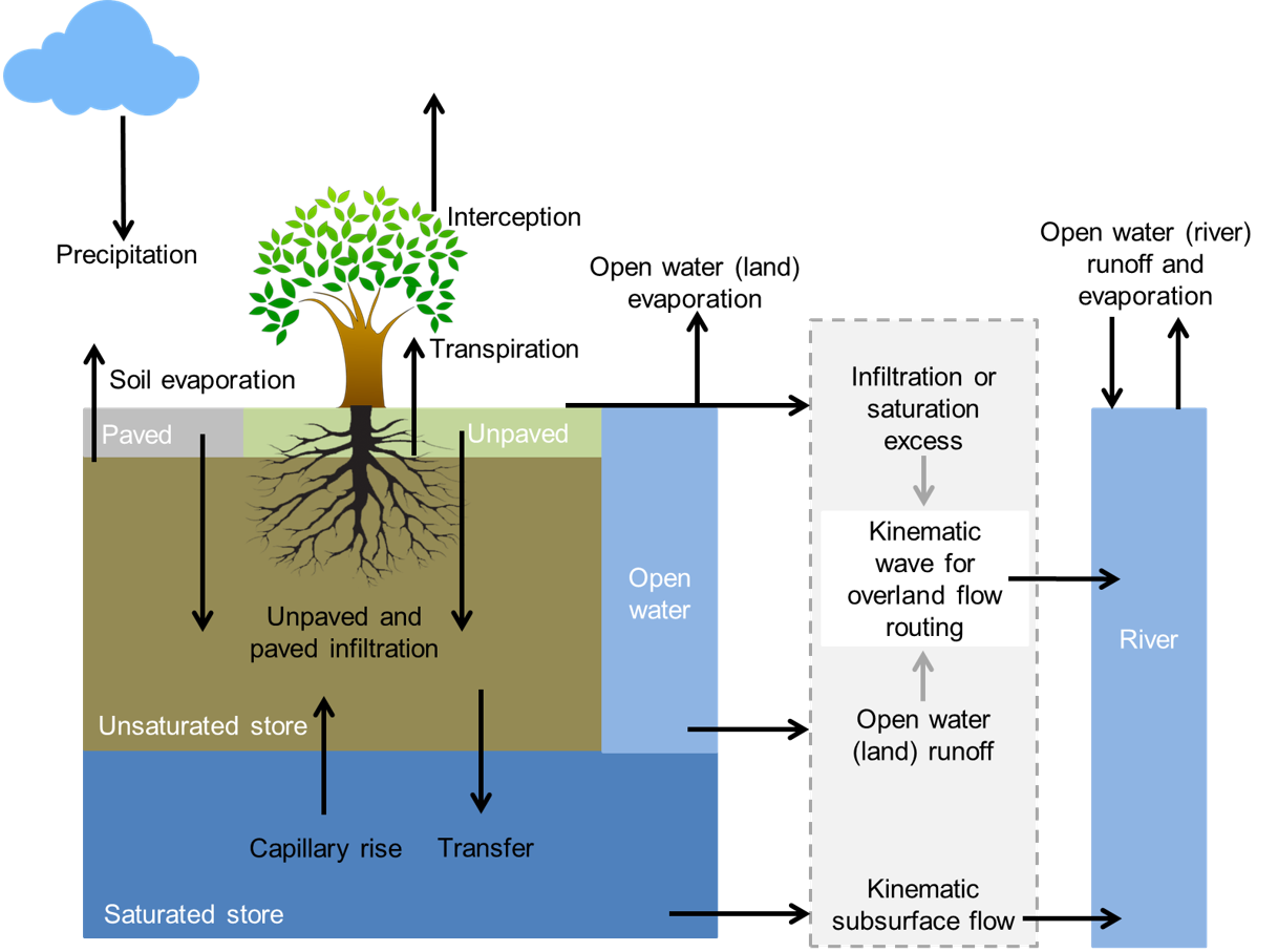
_images/wflow_sbm_soil.png — Overview of the different processes and fluxes in the wflow_sbm model.¶

Limitations¶

The wflow_sbm concept has been developed steep catchments and relatively thin soils. In addition, the numerical solution of the soil water flow is a simple explicit scheme and the lateral groundwater flow follows topography rather than true hydraulic head. Although the waterdem=1 option forces the model to recalculate the flow direction each timestep – thus giving a more realistic groundwater flow – the following limitation apply:

Results for deep soils > 2m may be unrealistic (also due to the simple representation of the unsaturated zone)
The lateral movement of groundwater may be very wrong in terrain that is not steep (use the waterdem=1 option)
The simple numerical solution means that results from a daily timestep model may be different from those with an hourly timestep. This can also cause water budget problems

Potential and Reference evaporation¶

The wflow_sbm model assumes the input to be potential evaporation. In many case the evaporation will be a reference evaporation for a different land cover. In that case you can use the et_reftopot.tbl file to set the mutiplication per landuse to go from the supplied evaporation to the potential evaporation for each land cover. By default al is set to 1.0 assuming the evaporation to be potential.

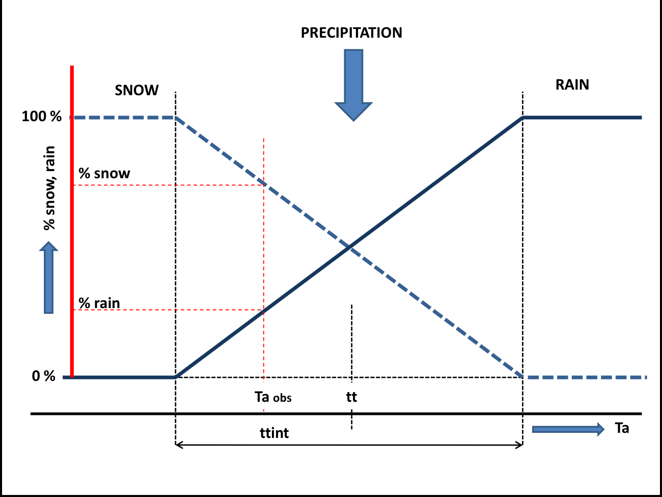
Snow¶

Precipitation enters the model via the snow routine. If the air temperature, $T_{a}$, is below a user-defined threshold $TT (\approx0^{o}C)$ precipitation occurs as snowfall, whereas it occurs as rainfall if $T_{a}\geq TT$. A another parameter $TTI$ defines how precipitation can occur partly as rain of snowfall (see the figure below). If precipitation occurs as snowfall, it is added to the dry snow component within the snow pack. Otherwise it ends up in the free water reservoir, which represents the liquid water content of the snow pack. Between the two components of the snow pack, interactions take place, either through snow melt (if temperatures are above a threshold $TT$) or through snow refreezing (if temperatures are below threshold $TT$). The respective rates of snow melt and refreezing are:

\[ \begin{align}\begin{aligned}Q_{m} = cfmax(T_{a}-TT)\;\;;T_{a}>TT\\Q_{r} = cfmax*cfr(TT-T_{a})\;;T_{a}<TT\end{aligned}\end{align} \]

where $Q_{m}$ is the rate of snow melt, $Q_{r}$ is the rate of snow refreezing, and $cfmax$ and $cfr$ are user defined model parameters (the melting factor $mm/(^{o}C*day)$ and the refreezing factor respectively)

Note

The FoCFMAX parameter from the original HBV version is not used. instead the CFMAX is presumed to be for the landuse per pixel. Normally for forested pixels the CFMAX is 0.6 {*} CFMAX

The air temperature, $T_{a}$, is related to measured daily average temperatures. In the original HBV-concept, elevation differences within the catchment are represented through a distribution function (i.e. a hypsographic curve) which makes the snow module semi-distributed. In the modified version that is applied here, the temperature, $T_{a}$, is represented in a fully distributed manner, which means for each grid cell the temperature is related to the grid elevation.

The fraction of liquid water in the snow pack (free water) is at most equal to a user defined fraction, $WHC$, of the water equivalent of the dry snow content. If the liquid water concentration exceeds $WHC$, either through snow melt or incoming rainfall, the surpluss water becomes available for infiltration into the soil:

\[Q_{in}=max\{(SW-WHC*SD);\;0.0\}\]

where $Q_{in}$ is the volume of water added to the soil module, $SW$ is the free water content of the snow pack and $SD$ is the dry snow content of the snow pack.

_images/hbv-snow.png — Schematic view of the snow routine¶

The snow model als has an optional (experimental) ‘mass-wasting’ routine. This transports snow downhill using the local drainage network. To use it set the variable MassWasting in the model section to 1.

# Masswasting of snow
# 5.67 = tan 80 graden
SnowFluxFrac = min(0.5,self.Slope/5.67) * min(1.0,self.DrySnow/MaxSnowPack)
MaxFlux = SnowFluxFrac * self.DrySnow
self.DrySnow = accucapacitystate(self.TopoLdd,self.DrySnow, MaxFlux)
self.FreeWater = accucapacitystate(self.TopoLdd,self.FreeWater,SnowFluxFrac * self.FreeWater )

Glaciers¶

If snow modeling is enabled Glacier modelling can also be enabled by including the following three entries in the modelparameters section:

::: [modelparameters] GlacierFrac=staticmaps/GlacierFrac.map,staticmap,0.0,0 G_TT=intbl/G_TT.tbl,tbl,0.0,1,staticmaps/GlacierFrac.map G_Cfmax=intbl/G_Cfmax.tbl,tbl,3.0,1,staticmaps/GlacierFrac.map

GlacierFrac is a map that gives the fraction of each grid cell covered by a glacier as a number between zero and one. Furthermore two lookup tables must be defined: G_TT and G_Cfmax. If the air temperature, $T_{a}$, is below $G\_TT (\approx0^{o}C)$ precipitation occurs as snowfall, whereas it occurs as rainfall if $T_{a}\geq G\_TT$.

With this the rate of glacier melt in mm is estimated as:

\[Q_{m} = G\_Cfmax(T_{a}-G\_TT)\;\;;T_{a}>G\_TT\]

where $Q_{m}$ is the rate of glacier meltand G_$Cfmax$ is the melting factor in $mm/(^{o}C*day)$.

Accumulated snow on top of the glacier is converted to ice (and will thus become part of the glacier store) if the total snow depth > 8300 mm. An S-curve is used to smooth the transition. A maximum of 8mm/day can be converted to ice.

(Source code)

Becuase the glacier store (GlacierStore.map) cannot be initialized by running the model a couple of year a default initial state map should be supplied by placing a GlacierStore.map file in the staticmaps directory. This map gives the amount of water (in mm) within the Glaciers at each gridcell)

The rainfall interception model¶

The analytical (Gash) model¶

The analytical model of rainfall interception is based on Rutter’s numerical model. The simplifications that introduced allow the model to be applied on a daily basis, although a storm-based approach will yield better results in situations with more than one storm per day. The amount of water needed to completely saturate the canopy is defined as:

\[P'=\frac{-\overline{R}S}{\overline{E}_{w}}ln\left[1-\frac{\overline{E}_{w}}{\overline{R}}(1-p-p_{t})^{-1}\right]\]

where $\overline{R}$ is the average precipitation intensity on a saturated canopy and $\overline{E}_{w}$ the average evaporation from the wet canopy and with the vegetation parameters $S$, $p$ and $p_t$ as defined previously. The model uses a series of expressions to calculate the interception loss during different phases of a storm. An analytical integration of the total evaporation and rainfall under saturated canopy conditions is then done for each storm to determine average values of $\overline{E}_{w}$ and $\overline{R}$. The total evaporation from the canopy (the total interception loss) is calculated as the sum of the components listed in the table below. Interception losses from the stems are calculated for days with $P\geq S_{t}/p_{t}$. $p_t$ and $S_t$ are small and neglected in the wflow_sbm model.

Table: Formulation of the components of interception loss according to Gash:

For $m$ small storms ($P_{g}<{P'}_{g}$)	$(1-p-p_{t})\sum_{j=1}^{m}P_{g,j}$
Wetting up the canopy in $n$ large storms ($P_{g}\geq{P'}_{g}$)	$n(1-p-p_{t}){P'}_{g}-nS$
Evaporation from saturated canopy during rainfall	$\overline{E}/\overline{R}\sum_{j=1}^{n}(P_{g,j}-{P'}_{g})$
Evaporation after rainfall ceases for $n$ large storms	$nS$
Evaporation from trunks in $q$ storms that fill the trunk storage	$qS_{t}$
Evaporation from trunks in ($m+n-q$) storms that do not fill the trunk storage	$p_{t}\sum_{j=1}^{m+n-q}P_{g,j}$

In applying the analytical model, saturated conditions are assumed to occur when the hourly rainfall exceeds a certain threshold. Often a threshold of 0.5 mm/hr is used. $\overline{R}$ is calculated for all hours when the rainfall exceeds the threshold to give an estimate of the mean rainfall rate onto a saturated canopy.

Gash (1979) has shown that in a regression of interception loss on rainfall (on a storm basis) the regression coefficient should equal to $\overline{E}_w/\overline{R}$. Assuming that neither $\overline{E}_w$ nor $\overline{R}$ vary considerably in time, $\overline{E}_w$ can be estimated in this way from $\overline{R}$ in the absence of above-canopy climatic observations. Values derived in this way generally tend to be (much) higher than those calculated with the penman-monteith equation.

Running with parameters derived from LAI¶

The model can determine the Gash parameters from an LAI maps. In order to switch this on you must define the LAI variable to the model (as in the example below).

[modelparameters]
LAI=inmaps/clim/LAI,monthlyclim,1.0,1
Sl=inmaps/clim/LCtoSpecificLeafStorage.tbl,tbl,0.5,1,inmaps/clim/LC.map
Kext=inmaps/clim/LCtoSpecificLeafStorage.tbl,tbl,0.5,1,inmaps/clim/LC.map
Swood=inmaps/clim/LCtoBranchTrunkStorage.tbl,tbl,0.5,1,inmaps/clim/LC.map

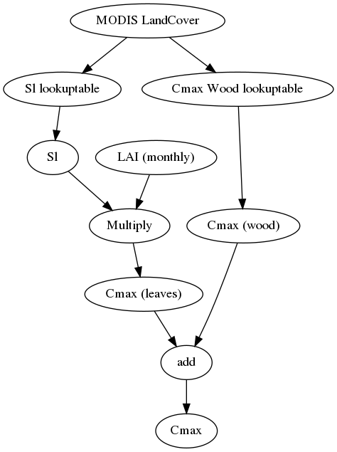
Here LAI refers to a MAP with LAI (in this case one per month), Sl to a lookuptable result of land cover to specific leaf storage, Kext to a lookuptable result of land cover to extinction coefficient and Swood to a lookuptable result of “canopy” capacity of the vegetation woody fraction.

Here it is assumed that Cmax(leaves) (Gash’ canopy capacity for the leaves only) relates linearly with LAI (c.f. Van Dijk and Bruijnzeel 2001). This done via the Sl (specific leaf storage). Sl is determined via a lookup table with land cover. Next the Cmax(leaves) is determined using:

\[Cmax(leaves) = Sl * LAI\]

The table below shows lookup table for Sl (as determined from Pitman 1986, Lui 1998).

 0           Water
 0.045   Evergreen Needle leaf Forest
 0.036   Evergreen Broadleaf Forest
 0.045   Deciduous Needle leaf Forest
 0.036   Deciduous Broadleaf Forest
 0.03926 Mixed Forests
 0.07    Closed Shrublands
 0.07    Open Shrublands
 0.07    Woody Savannas
 0.09    Savannas
0.1272  Grasslands
0.1272  Permanent Wetland
0.1272  Croplands
0.04    Urban and Built-Up
0.1272  Cropland/Natural Vegetation Mosaic
0.0         Snow and Ice
0.04    Barren or Sparsely Vegetated

To get to total storage (Cmax) the woody part of the vegetation also needs to be added. This is done via a simple lookup table between land cover the Cmax(wood):

digraph cmax {
"MODIS LandCover" -> "Sl lookuptable";
"Sl lookuptable" -> Sl -> Multiply;
"LAI (monthly)" -> Multiply -> "Cmax (leaves)" -> add;
"MODIS LandCover" -> "Cmax Wood lookuptable";
"Cmax Wood lookuptable" -> "Cmax (wood)";
"Cmax (wood)"-> add;
add -> Cmax;
}

The table below relates the land cover map to the woody part of the Cmax.

 0           Water
 0.5     Evergreen Needle leaf Forest
 0.5         Evergreen Broadleaf Forest
 0.5         Deciduous Needle leaf Forest
 0.5         Deciduous Broadleaf Forest
 0.5         Mixed Forests
 0.2         Closed Shrublands
 0.1         Open Shrublands
 0.2         Woody Savannas
 0.01    Savannas
0.0         Grasslands
0.01    Permanent Wetland
0.0         Croplands
0.01    Urban and Built-Up
0.01    Cropland/Natural Vegetation Mosiac
0.0         Snow and Ice
0.04    Barren or Sparsely Vegetated

The canopy gap fraction is determined using the k: extinction coefficient (van Dijk and Bruijnzeel 2001):

\[CanopyGapFraction = exp(-k * LAI)\]

The table below show how k is related to land cover:

 0.7     Water
 0.8     Evergreen Needle leaf Forest
 0.8     Evergreen Broadleaf Forest
 0.8     Deciduous Needle leaf Forest
 0.8     Deciduous Broadleaf Forest
 0.8     Mixed Forests
 0.6     Closed Shrublands
 0.6     Open Shrublands
 0.6     Woody Savannas
 0.6     Savannas
0.6     Grasslands
0.6     Permanent Wetland
0.6     Croplands
0.6     Urban and Built-Up
0.6     Cropland/Natural Vegetation Mosaic
0.6     Snow and Ice
0.6     Barren or Sparsely Vegetated

The modified rutter model¶

For subdaily timesteps the model uses a simplification of the Rutter model. The simplified model is solved explicitly and does not take drainage from the canopy into account.

def rainfall_interception_modrut(Precipitation,PotEvap,CanopyStorage,CanopyGapFraction,Cmax):
   """
   Interception according to a modified Rutter model. The model is solved
   explicitly and there is no drainage below Cmax.

   Returns:
       - NetInterception: P - TF - SF (may be different from the actual wet canopy evaporation)
       - ThroughFall:
       - StemFlow:
       - LeftOver: Amount of potential eveporation not used
       - Interception: Actual wet canopy evaporation in this thimestep
       - CanopyStorage: Canopy storage at the end of the timestep

   """

   ##########################################################################
   # Interception according to a modified Rutter model with hourly timesteps#
   ##########################################################################

   p = CanopyGapFraction
   pt = 0.1 * p

   # Amount of P that falls on the canopy
   Pfrac = (1 - p -pt) * Precipitation

   # S cannot be larger than Cmax, no gravity drainage below that
   DD = ifthenelse (CanopyStorage > Cmax , Cmax - CanopyStorage , 0.0)
   self.CanopyStorage = CanopyStorage - DD

   # Add the precipitation that falls on the canopy to the store
   CanopyStorage = CanopyStorage + Pfrac

   # Now do the Evap, make sure the store does not get negative
   dC = -1 * min(CanopyStorage, PotEvap)
   CanopyStorage = CanopyStorage + dC

   LeftOver = PotEvap +dC; # Amount of evap not used


   # Now drain the canopy storage again if needed...
   D = ifthenelse (CanopyStorage > Cmax , CanopyStorage - Cmax , 0.0)
   CanopyStorage = CanopyStorage - D

   # Calculate throughfall
   ThroughFall = DD + D + p * Precipitation
   StemFlow = Precipitation * pt

   # Calculate interception, this is NET Interception
   NetInterception = Precipitation - ThroughFall - StemFlow
   Interception = -dC

   return NetInterception, ThroughFall, StemFlow, LeftOver, Interception, CanopyStorage

The soil model¶

Infiltration¶

If the surface is (partly) saturated the rainfall that falls onto the saturated area is added to the surface runoff component. Infiltration of the remaining water is determined as follows:

First the soil infiltration capacity is adjusted in case the soil is frozen. The remaining storage capacity of the unsaturated store is determined. The infiltrating water is split is two parts, the part that falls on compacted areas and the part that falls on non-compacted areas. First the amount of water that infiltrates in non-compacted areas is calculated by taking the minimum of the remaining storage capacity, the maximum soil infiltration rate and the water on non-compacted areas. After adding the infiltrated water to the unsaturated store the same is done for the compacted areas after updating the remaining storage capacity.

The wflow_sbm soil water accounting scheme¶

A detailed description of the SBM model has been given by [vertessy]. Briefly: the soil is considered as a bucket with a certain depth ($z_{t}$), divided into a saturated store ($S$) and an unsaturated store ($U$), the magnitudes of which are expressed in units of depth. The top of the $S$ store forms a pseudo-water table at depth $z_{i}$ such that the value of $S$ at any time is given by:

\[S=(z_{t}-z_{i})(\theta_{s}-\theta_{r})\]

where:

$\theta_{s}$ and $\theta_{r}$ are the saturated and residual soil water contents, respectively.

The unsaturated store ($U$) is subdivided into storage ($U_{s}$) and deficit ($U_{d}$) which are again expressed in units of depth:

\[ \begin{align}\begin{aligned}U_{d}=(\theta_{s}-\theta_{r})z_{i}-U\\U_{s}=U-U_{d}\end{aligned}\end{align} \]

The saturation deficit ($S_{d}$) for the soil profile as a whole is defined as:

\[S_{d}=(\theta_{s}-\theta_{r})z_{t}-S\]

All infiltrating rainfall enters the $U$ store first. The transfer of water from the $U$ store to the $S$ store ($st$) is controlled by the saturated hydraulic conductivity {} at depth $z_{i}$ and the ratio between $U$ and $S_{d}$:

\[st=K_{\mathit{sat}}\frac{U_{s}}{S_{d}}\]

Hence, as the saturation deficit becomes smaller, the rate of the transfer between the $U$ and $S$ stores increases.

_images/wflow_soil.png — Schematisation of the soil within the wflow_sbm model¶

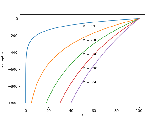
Saturated conductivity ($K_{sat}$) declines with soil depth ($z$) in the model according to:

where:

$K_{0}$ is the saturated conductivity at the soil surface and

$f$ is a scaling parameter [$m^{-1}$]

The scaling parameter $f$ is defined by:

$f=\frac{\theta_{s}-\theta_{r}}{M}$

with $\theta_{s}$ and $\theta_{r}$ as defined previously and $M$ representing a model parameter (expressed in meters).

Figure: Plot of the relation between depth and conductivity for different values of M

(Source code, png, hires.png, pdf)

The $S$ store can be drained laterally via subsurface flow according to:

$sf=K_{0}\mathit{tan}(\beta)e^{-S_{d}/M}$

where:

$\beta$ is element slope angle [deg.]

$sf$ is the calculated subsurface flow [$m^{2}d^{-1}$]

$S_{d}$ is the saturation deficit defined as: ($(\theta_{s}-\theta_{r})z_{t}-S$)

with $M$ and $S_{d}$ as defined previously. A schematic representation of the various hydrological processes and pathways modelled by SBM (infiltration, exfiltration, Hortonian and saturation overland flow, subsurface flow) is provided by Vertessy (1999).

Transpiration and soil evaporation¶

The potential eveporation left over after the interception is split in potential soil evaporation and potential transpiration base on the canopy gap fraction (assumed to be identical to the amount of bare soil).

Soi evaporation is scaled according to:

$soilevap = potensoilevap * SaturationDeficit/SoilWaterCapacity$

As such, evaporation will be potential if the soil is fully wetted and it decreases linear with increasing soil moisture deficit.

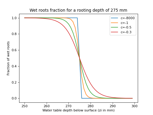
The original SBM model does not include transpiration or a notion of capilary rise. In wflow_sbm transpiration is first taken from the $S$ store if the roots reach the water table $z_{i}$. If the $S$ store cannot satisfy the demand the $U$ store is used next. First the number of wet roots is determined (going from 1 to 0) using an sigmoid function as follows:

\[WetRoots = 1.0/(1.0 + e^{-SharpNess (WaterTable - RootingDepth)})\]

Here the sharpness parameter (by default a large negative value, -80000.0) parameter determines if there is a stepwise output or a more gradual output (default is stepwise). WaterTable is the level of the Water table in the gridcell in mm below the surface, RootingDepth is the maximum depth of the roots also in mm below the surface. For all values of WaterTable smaller that RootingDepth a value of 1 is returned if they are equal a value of 0.5 is returned if the WaterTable is larger than the RootingDepth a value of 0 is returned. The returned WetRoots fraction is multiplied by the potential evaporation (and limited by the available water in saturated zone) to get the transpiration from the saturated part of the soil.

Figure: Plot showing the fraction of wet roots for different values of c for a RootingDepth of 275mm

(Source code, png, hires.png, pdf)

Next the remaining potential evaporation is used to extract water from the unsaturated store:

wetroots = sCurve(WTable, a=RootingDepth, c=smoothpar)
ActEvapSat = min(PotTrans * wetroots, SatWaterDepth)
SatWaterDepth = SatWaterDepth - ActEvapSat
RestPotEvap = PotTrans - ActEvapSat

# now try unsat store
AvailCap = max(0.0,ifthenelse(WTable < RootingDepth,  cover(1.0),  RootingDepth/(WTable + 1.0)))
MaxExtr = AvailCap * UStoreDepth
ActEvapUStore = min(MaxExtr, RestPotEvap, UStoreDepth)
UStoreDepth = UStoreDepth - ActEvapUStore

ActEvap = ActEvapSat + ActEvapUStore

Remaining evaporative demand is split between evaporation of open water and soil evaporation. This first amount is subtracted from the water that would otherwise enter the kinematic wave.

Capilary rise is determined using the following approach: first the $K_{sat}$ is determined at the water table $z_{i}$; next a potential capilary rise is determined from the minimum of the $K_{sat}$, the actual transpiration taken from the $U$ store, the available water in the $S$ store and the deficit of the $U$ store. Finally the potential rise is scaled using the distance between the roots and the water table using:

$CS=CSF/(CSF+z_{i}-RT)$

in which $CS$ is the scaling factor to multiply the potential rise with, $CSF$ is a model parameter (default = 100, use CapScale.tbl to set differently) and $RT$ the rooting depth. If the roots reach the water table ($RT>z_{i}$) $CS$ is set to zero thus setting the capilary rise to zero.

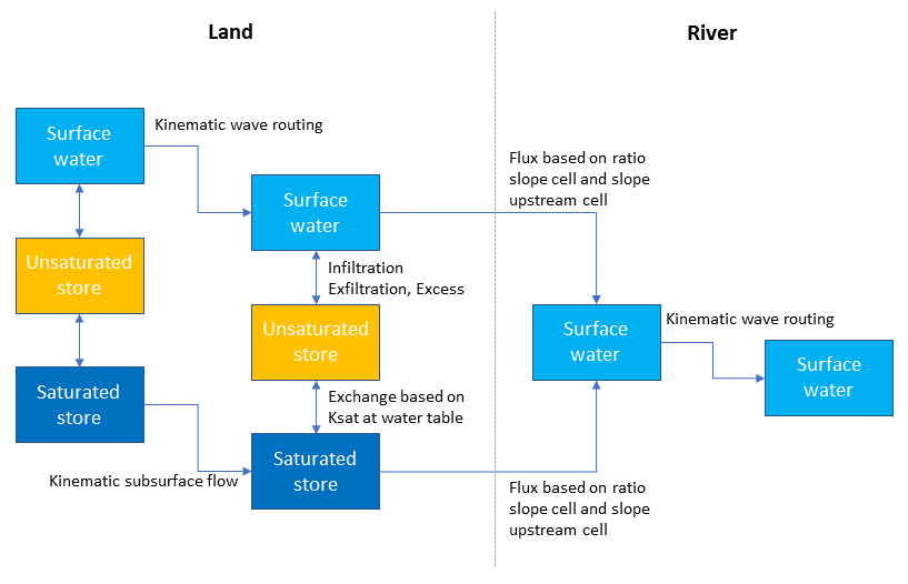
Water in the saturated store is transferred laterally along the DEM using the following steps:
1. a maximum flux for each cell is determined by determining the {} over the saturated part and the available water in each cell
2. water is routed downslope (using the PCRaster accucapacityflux operator) by multiplying the {} by the slope and limiting the flux maximum determined in the previous step
3. the program can either use the DEM to route the water or (more appropriate in flat areas) the actual slope of the water table. The latter option slows down the program considerably
surplus water in cells as a result of the previous step is added to the kinematic wave reservoir

Leakage¶

If the MaxLeakage parameter may is set > 0 water is lost from the Saturated zone and runs out of the model.

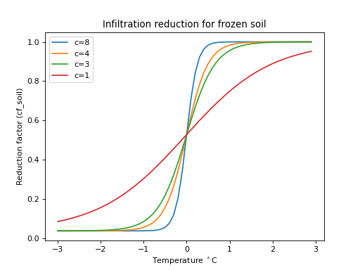
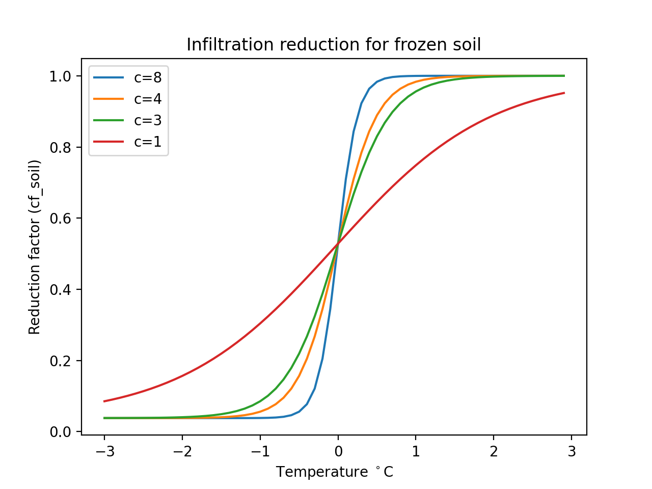
Soil temperature¶

The near surface soil temperature is modelled using a simple equation [Wigmosta]:

\[T_s^{t} = T_s^{t-1} + w (T_a - T_s^{t-1})\]

where $T_s^{t}$ is the near-surface soil temperature at time t, $T_a$ is air temperature and $w$ is a weighting coefficient determined through calibration (default is 0.1125 for daily timesteps, 0.9 for 3-hourly timesteps)

if T_s < 0 than a K_{sat} reduction factor (default 0.038) is applied. An S-curve (see plot below) is used to make a smooth transition (a c-factor of 8 is used).

(Source code, png, hires.png, pdf)

Sub-grid runoff generation¶

Sub-grid runoff generaten can be switched on on off in the configuration file. In general this feature is used if the grid cell size is relatively larger compared to the variation of topography. In addition you will need to have information on the distribution of altitude within a grid-cell. Depending on the topography sub-grid runoff generation may be useful around 1x1km and larger.

The basis is formed by a sigmoid ($S$) function that is fitted using a 10, 50 and 90 percentile DEM. The $S$ function is defined as:

\[S = 1.0/(b + e^{(-c (X - a))})\]

Where:

X = input variable (in this case the absolute scaled groundwater level)

b = 1.0

c = sharpness parameter. Higher values give sharper step

a = centre-point of the curve (normally the 50% DEM)

The $c$ parameter is estimated by reversing the function above to:

\[c = log(1.0/p - 1)/(dem_{p} - dem_{50})\]

where:

percentile is the percentile of $dem_{p}$

$dem_{50}$ is the average altitude in the gridcell

$dem_{p}$ is the altitude below with percentile (p) cells of the dem are found

The outcome of the $S$ will range from 0 to 1 for inputs ranging from the minimum altitude to the maximum altitude (within the gridcell). Thereore, the calculated groundwater levels within the cell are scale to match the minimum and maximum altitude within the cell using:

\[G_s = (A_{max}-A_{min})/FZT/GWPerc\]

where:

$G_s$ is the scaling factor

$A_{max}$ the maximum altitude within the cell

$A_{min}$ the minumum altitude within the cell

$FZT$ the total thickness of the soil in the model

$GWperc$ is a dimensionless parameter (from >0 to 1) that determines which part of the soil profile generates runoff. If it is 1 runoff is generated whenever there is groundwater in the system. If it is 0.1 only the top 10 % of the soil profile generated runoff

self.DemMax=readmap(self.Dir + "/staticmaps/wflow_demmax")
self.DrainageBase=readmap(self.Dir + "/staticmaps/wflow_demmin")
self.CC = min(100.0,-log(1.0/0.1 - 1)/min(-0.1,self.DrainageBase - self.Altitude))
self.GWScale = (self.DemMax-self.DrainageBase)/self.SoilThickness / self.RunoffGeneratingGWPerc

Note

The model determines the C for the upper half and the lower half of the curve: seperate and averages the results.

Warning

This is an poorly tested feature

In the dynamic section of the model the absolute groundwater level is determined and scaled before it is fed into the $S$ curve function. The result is a estimated saturated fraction within a the gridcell. The saturated fraction is used to generated Saturation Overland Flow (SOF) and generate ouflow from the groundwater reservoir:

The saturated conductivity for the average groundwaterlevel is determined
The available water at the surface is multiplied by the saturated fraction and added to the kinematic wave reservoir (SOF)
Outflow from the groundwater reservoir is determined using average slope multiplied by the conductivity and the saturated fraction limited by the amount of water in the groundwater reservoir.

in dynamic:

self.AbsoluteGW = self.DemMax - (self.zi * self.GWScale)
# Determine saturated fraction of cell
self.SubCellFrac = sCurve(self.AbsoluteGW, c=self.CC, a=self.Altitude + 1.0)
# Make sure total of SubCellFRac + WaterFRac + RiverFrac <=1 to avoid double counting
Frac_correction = ifthenelse((self.SubCellFrac + self.RiverFrac + self.WaterFrac) > 1.0,
                                         self.SubCellFrac + self.RiverFrac + self.WaterFrac - 1.0, 0.0)
self.SubCellRunoff = (self.SubCellFrac - Frac_correction) * self.AvailableForInfiltration
self.SubCellGWRunoff = min(self.SubCellFrac * self.SatWaterDepth,
                           max(0.0,self.SubCellFrac * self.Slope * self.KsatVer * \
                               self.KsatHorFrac * exp(-self.f * self.zi)))

Irrigation and water demand¶

Water demand (surface water only) by irrigation can be configured in two ways:

By specifying the water demand externally (as a lookup table, series of maps etc)
By defining irrigation areas. Within those areas the demand is calculated as the difference between potential ET and actual transpiration

For both options a fraction of the supplied water can be put back into the river at specified locations

The following maps and variables can be defined:

wflow_irrigationareas.map:

Map of areas where irrigation is applied. Each area has a unique id. The areas do not need to be continuous but all cells with the same id are assumed to belong to the same irrigation area.

wflow_irrisurfaceintake.map:

Map of intake points at the river(s). The id of each point should correspond to the id of an area in the wflow_irrigationareas map.

wflow_irrisurfacereturns.map:

Map of water return points at the river(s). The id of each point should correspond to the id of an area in the wflow_irrigationareas map or/and the wflow_irrisurfaceintake.map.

IrriDemandExternal:

Irrigation demand supplied to the model. This can be doen by adding an entry to the modelparameters section. if this is doen the irrigation demand supplied here is used and it is NOT determined by the model. Water demand should be given with a negative sign! See below for and example entry in the modelparameters section:

IrriDemandExternal=intbl/IrriDemandExternal.tbl,tbl,-34.0,0,staticmaps/wflow_irrisurfaceintakes.map

In this example the default demand is $-34 m^3/s$. The demand must be linked to the map wflow_irrisurfaceintakes.map. Alternatively we can define this as a timeseries of maps:

IrriDemandExternal=/inmaps/IRD,timeseries,-34.0,0

DemandReturnFlowFraction:

Fraction of the supplied water the returns back into the river system (between 0 and 1). This fraction must be supplied at the wflow_irrisurfaceintakes.map locations but the water that is returned to the river will be returned at the wflow_irrisurfacereturns.map locations. If this variable is not defined the default is 0.0. See below for an example entry in the modelparameters section:

DemandReturnFlowFraction=intbl/IrriDemandReturn.tbl,tbl,0.0,0,staticmaps/wflow_irrisurfaceintakes.map

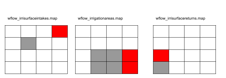
_images/wflow_irrigation.png — Figure showing the three maps that define the irrigation intake points areas and return flow locations.¶

The irrigation model can be used in the following two modes:

An external water demand is given (the user has specified the IrriDemandExternal variable). In this case the demand is enforced. If a matching irrigation area is found the supplied water is converted to an amount in mm over the irrigation area. The supply is converted in the next timestep as extra water available for infiltration in the irrigation area. If a DemandReturnFlowFraction is defined this fraction is the supply is returned to the river at the wflow_irrisurfacereturns.map points.
Irrigation areas have been defined and no IrriDemandExternal has been defined. In this case the model will estimate the irrigation water demand. The irrigation algorithim works as follows: For each of the areas the difference between potential transpiration and actual transpiration is determined. Next, this is converted to a demand in $m^3/s$ at the corresponding intake point at the river. The demand is converted to a supply (taking into account the available water in the river) and converted to an amount in mm over the irrigation area. The supply is converted in the next timestep as extra water available for infiltration in the irrigation area. This option has only be tested in combination with a monthly LAI climatology as input. If a DemandReturnFlowFraction is defined this fraction is the supply is returned to the river at the wflow_irrisurfacereturns.map points.

Bifurcations¶

A PCRaster local drainage direction (ldd) map only allows for one downstream neighbour cell. Bifurcations can be included in WFlow by providing the following files:

wflow_bifurcations.map:: PCRaster ordinal map, identifying all bifurcations; cells having two downstream neighbours, of which only on is represented by the ldd.
wflow_bifurcations_ds.map:: PCRaster ordinal map, identifying the locations in the bifurcation canal to which a part of the main river runoff (self.SurfaceRunoff), at the location of bifurcation, is to be diverted to. The IDs in this map match the IDs in wflow_bifurcations.map
Bifurcations.tbl:: a table with the part of the discharge (self.SurfaceRunoff) at the location of the bifurcation, specified in wflow_bifurcations.map, which is diverted to the location specified in wflow_bifurcations_ds.map. The table consists of two columns: (1) a column with the bifurcation ID matching the IDs in both map-files and (2) the part of self.SurfaceRunoff at the bifurcation to be diverted to the bifurcation canal at the location specified in wflow_bifurcations_ds.map.

Example of a tbl-file:

1 0.5
2 0.3

The locations in wflow_bifurcations.map are interpreted as sinks, where a part of the total flow will be extracted. The locations in wflow_bifurcations_ds.map are interpreted as sources, where a the extracted part will be supplied.

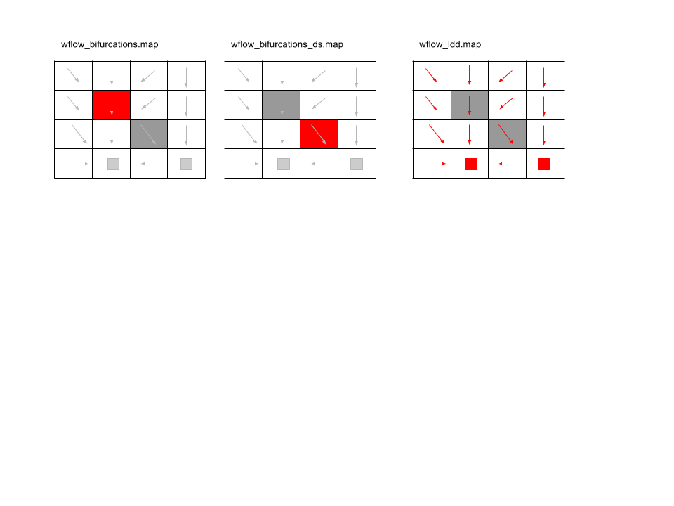
_images/wflow_bifurcation.png — Figure showing (left) wflow_bifurcations.map, (middle) wflow_bifurcations_ds.map, (right) wflow_ldd.map¶

Kinematic wave and River Width¶

The river width is determined from the DEM the upstream area and yearly average discharge ([Finnegan]):

The early average Q at outlet is scaled for each point in the drainage network with the upstream area. $\alpha$ ranges from 5 to > 60. Here 5 is used for hardrock, largre values are used for sediments

Implementation:

upstr = catchmenttotal(1, self.TopoLdd)
Qscale = upstr/mapmaximum(upstr) * Qmax
W = (alf * (alf + 2.0)**(0.6666666667))**(0.375) * Qscale**(0.375) *\
     (max(0.0001,windowaverage(self.Slope,celllength() * 4.0)))**(-0.1875) *\
     self.N **(0.375)
RiverWidth = W

The table below list commonly used Manning’s N values (in the N_River .tbl file). Please note that the values for non river cells may arguably be set significantly higher. (Use N.tbl for non-river cells and N_River.tbl for river cells)

Manning’s N values¶
Type of Channel and Description	Minimum	Normal	Maximum
Main Channels
clean, straight, full stage, no rifts or deep pools	0.025	0.03	0.033
same as above, but more stones and weeds	0.03	0.035	0.04
clean, winding, some pools and shoals	0.033	0.04	0.045
same as above, but some weeds and stones	0.035	0.045	0.05
same as above, lower stages, more ineffective slopes and sections	0.04	0.048	0.055
same as second with more stones	0.045	0.05	0.06
sluggish reaches, weedy, deep pools	0.05	0.07	0.08
very weedy reaches, deep pools, or floodways with heavy stand of timber and underbrush	0.075	0.1	0.15
Mountain streams
bottom: gravels, cobbles, and few boulders	0.03	0.04	0.05
bottom: cobbles with large boulders	0.04	0.05	0.07

Subcatchment flow¶

Normally the the kinematic wave is continuous throughout the model. By using the the SubCatchFlowOnly entry in the model section of the ini file all flow is at the subcatchment only and no flow is transferred from one subcatchment to another. This can be handy when connecting the result of the model to a water allocation model such as Ribasim.

Example:

[model]
SubCatchFlowOnly = 1

Model variables stores and fluxes¶

The diagram below shows the stores and fluxes in the model in terms of internal variable names. It onlys shows the soil and Kinematic wave reservoir, not the canopy model.

$digraph grids { compound=true; node[shape=record]; UStoreDepth [shape=box]; OutSide [style=dotted]; SoilWaterDepth [shape=box]; UStoreDepth -> SoilWaterDepth [label="Transfer [mm]"]; SoilWaterDepth -> UStoreDepth [label="CapFlux [mm]"]; SoilWaterDepth ->KinematicWaveStore [label="ExfiltWaterCubic [m^3/s]"]; "OutSide" -> UStoreDepth [label="ActInfilt [mm]"]; UStoreDepth -> OutSide [label="ActEvapUStore [mm]"]; SoilWaterDepth -> OutSide [label="ActEvap-ActEvapUStore [mm]"]; SoilWaterDepth -> KinematicWaveStore [label="SubCellGWRunoffCubic [m^3/s]"]; "OutSide" -> KinematicWaveStore [label="SubCellRunoffCubic [m^3/s]"]; "OutSide" -> KinematicWaveStore [label="RunoffOpenWater [m^3/s]"] ; "OutSide" -> KinematicWaveStore [label="FreeWaterDepthCubic [m^3/s]"] ; }$

Processing of meteorological forcing data¶

Although the model has been setup to do as little data processing as possible it includes an option to apply an altitude correction to the temperature inputs. The three squares below demonstrate the principle.

digraph grids {
node[shape=record];
a[label="{5|5|5}|{5|5|5}|{5|5|5}"];
b[label="{1|2|3}|{4|5|6}|{7|8|9}"];
c[label="{4|3|2}|{1|0|-1}|{-2|-3|-4}"];
"Average T input grid" -> a
"Correction per cell" -> b
"Resulting T" -> c
}

wflow_sbm takes the correction grid as input and applies this to the input temperature. The correction grid has to be made outside of the model. The correction grid is optional.

Note

The temperature correction map is specified in the model section of the ini file:

[model] TemperatureCorrectionMap=NameOfTheMap

If the entry is not in the file the correction will not be applied

Guidelines for wflow_sbm model parameters¶

The tables below shows the most important parameters and suggested ranges

CanopyGapFraction file:///media/schelle/BIG/LINUX/wflow/cases/maas/intbl/Cfmax.tbl

EoverR - Ratio of average wet canopy evaporation rate over precipitation rate - usually between 0.06 and 0.15 depending on climate and site.
FirstZoneCapacity -

FirstZoneKsatVer.tbl
file:///media/schelle/BIG/LINUX/wflow/cases/maas/intbl/FirstZoneMinCapacity.tbl
file:///media/schelle/BIG/LINUX/wflow/cases/maas/intbl/InfiltCapPath.tbl
file:///media/schelle/BIG/LINUX/wflow/cases/maas/intbl/InfiltCapSoil.tbl
file:///media/schelle/BIG/LINUX/wflow/cases/maas/intbl/M.tbl
file:///media/schelle/BIG/LINUX/wflow/cases/maas/intbl/MaxCanopyStorage.tbl
file:///media/schelle/BIG/LINUX/wflow/cases/maas/intbl/MaxLeakage.tbl
file:///media/schelle/BIG/LINUX/wflow/cases/maas/intbl/N_River.tbl
file:///media/schelle/BIG/LINUX/wflow/cases/maas/intbl/N.tbl
file:///media/schelle/BIG/LINUX/wflow/cases/maas/intbl/RootingDepth.tbl
file:///media/schelle/BIG/LINUX/wflow/cases/maas/intbl/RunoffGeneratingGWPerc.tbl
file:///media/schelle/BIG/LINUX/wflow/cases/maas/intbl/thetaR.tbl
file:///media/schelle/BIG/LINUX/wflow/cases/maas/intbl/thetaS.tbl
file:///media/schelle/BIG/LINUX/wflow/cases/maas/intbl/TT.tbl
file:///media/schelle/BIG/LINUX/wflow/cases/maas/intbl/TTI.tbl
file:///media/schelle/BIG/LINUX/wflow/cases/maas/intbl/WHC.tbl

Beta.tbl: Beta parameter used in the kinematic wave function. Should be set to 0.6 (will be removed later)
CanopyGapFraction.tbl: Gash interception model parameter: the free throughfall coefficient.
EoverR.tbl: Gash interception model parameter. Ratio of average wet canopy evaporation rate over average precipitation rate.
FirstZoneCapacity.tbl: Maximum capacity of the saturated store [mm]
MaxLeakage.tbl: Maximum leakage [mm/day]. Leakage is lost to the model. Usually only used for i.e. linking to a dedicated groundwater model. Normally set to zero in all other cases.
FirstZoneKsatVer.tbl: Saturated conductivity of the store at the surface. The M parameter determines how this decreases with depth.
FirstZoneMinCapacity.tbl: Minimum capacity of the saturated store [mm]
InfiltCapPath.tbl: Infiltration capacity [mm/day] of the compacted soil (or paved area) fraction of each gridcell
InfiltCapSoil.tbl: Infiltration capacity [mm/day] of the non-compacted soil fraction (unpaved area) of each gridcell
M.tbl: Soil parameter determining the decrease of saturated conductivity with depth. Usually between 20 and 2000 (if the soil depth is in mm)
MaxCanopyStorage.tbl: Canopy storage [mm]. Used in the Gash interception model
N.tbl: Manning N parameter for the Kinematic wave function. Higher values dampen the discharge peak.
PathFrac.tbl: Fraction of compacted area per gridcell
RootingDepth.tbl: Rooting depth of the vegetation [mm]
thetaR.tbl: Residual water content
thetaS.tbl: Water content at saturation

Calibrating the wflow_sbm model¶

Introduction¶

As with all hydrological models calibration is needed for optimal performance. Currently we are working on getting the link with the OpenDA calibration environment running (not tested yet). We have calibrated the Rhine/Meuse models using simple shell scripts and the XX and XX command-line parameters to multiply selected model parameters and evaluate the results later.

Parameters¶

M: Once the depth of the soil has been set for the different land-use types the M parameter is the most important variable in calibrating the model. The decay of the conductivity with depth controls the baseflow resession and part of the stormflow curve.
N: The Manning N parameter controls the shape of the hydrograph (the peak parts). In general it is advised to set N to realistic values for the rivers, for the land phase higher values are usually needed.
Ksat: Increasing the Ksat will lower the hydrograph (baseflow) and flatten the peaks. The latter also depend on the shape of the catchment.
FirstZoneCapacity: Increasing the storage capacity of the soil will decrease the outflow
RunoffGeneratingGWPerc: Default is 0.1. Determines the (upper) part of the groudwater that can generate runoff in a cell. This is only used of the RunoffGenSigmaFunction option is set to 1. In general generating more runoff before a cell is completely saturated (which is the case if RunoffGenSigmaFunction is set to 0) will lead to more baseflow and flattening of the peaks.

Changes in hydrographs for different values of parameters¶

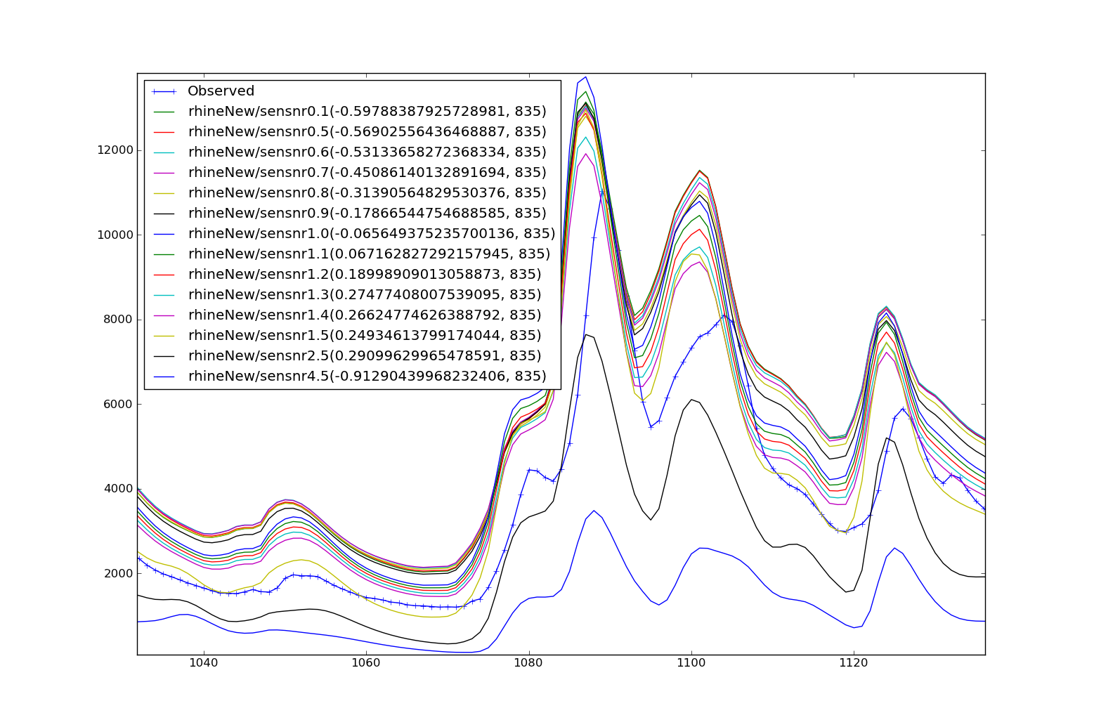
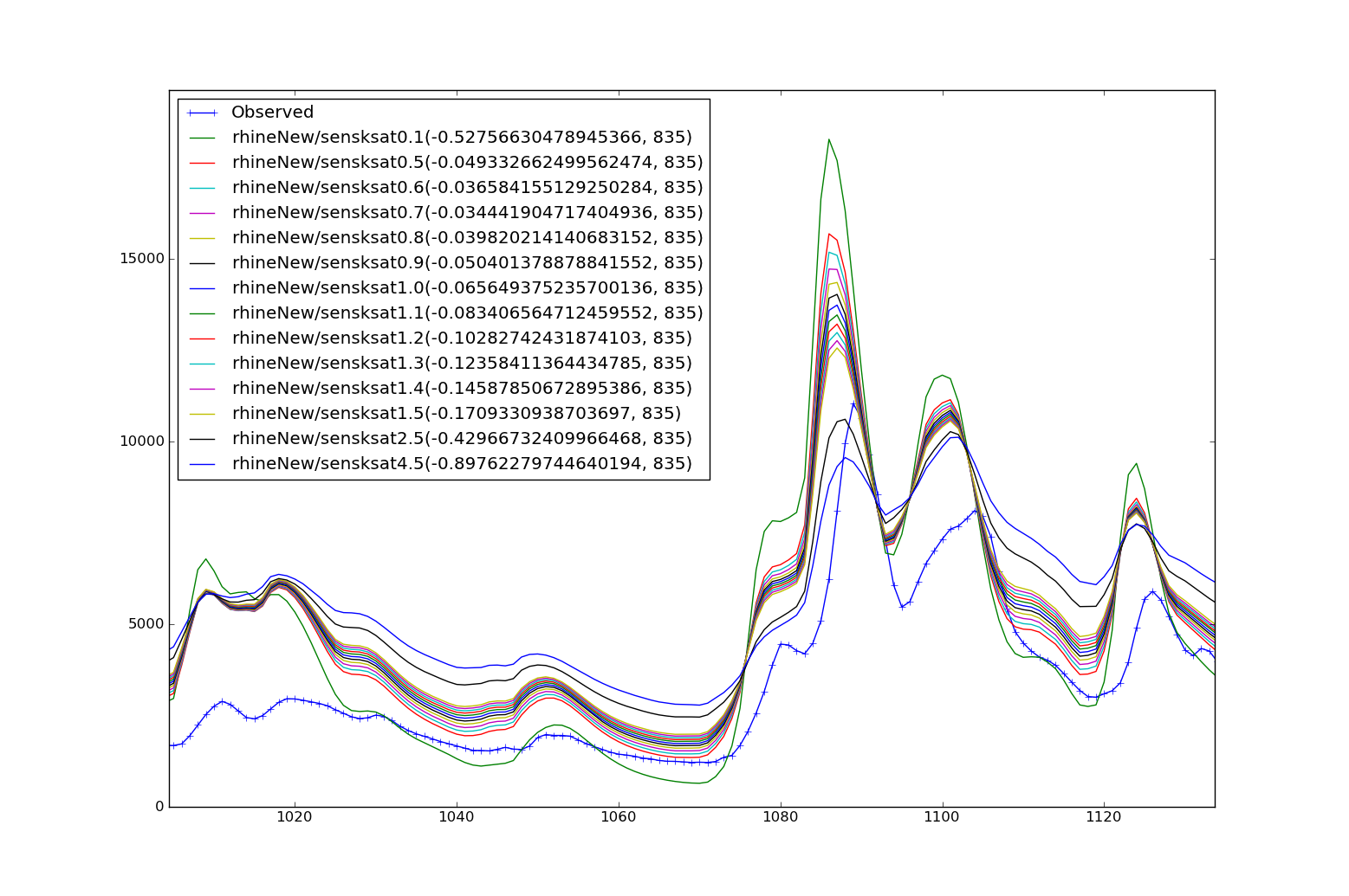
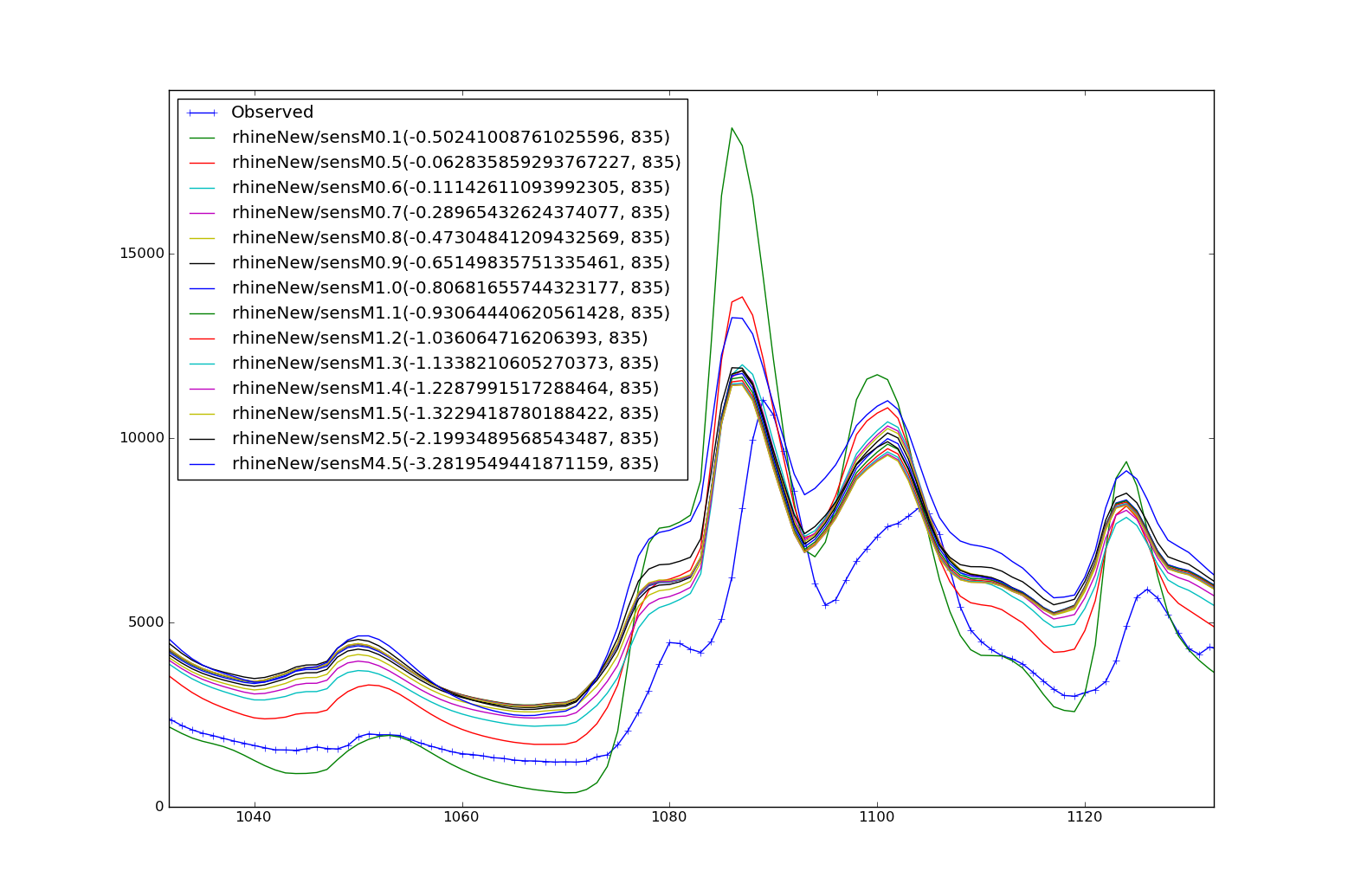
References¶

[vertessy]

Vertessy, R.A. and H. Elsenbeer, “Distributed modelling of storm flow generation in an Amazonian rainforest catchment: effects of model parameterization,” Water Resources Research, vol. 35, no. 7, pp. 2173–2187, 1999.

[Finnegan]

Noah J. Finnegan et al 2005 Controls on the channel width of rivers: Implications for modeling fluvial incision of bedrock”

[Wigmosta]

Wigmosta, M. S., L. J. Lane, J. D. Tagestad, and A. M. Coleman (2009), Hydrologic and erosion models to assess land use and management practices affecting soil erosion, Journal of Hydrologic Engineering, 14(1), 27-41.

For \(m\) small storms (\(P_{g}<{P'}_{g}\))	\((1-p-p_{t})\sum_{j=1}^{m}P_{g,j}\)
Wetting up the canopy in \(n\) large storms (\(P_{g}\geq{P'}_{g}\))	\(n(1-p-p_{t}){P'}_{g}-nS\)
Evaporation from saturated canopy during rainfall	\(\overline{E}/\overline{R}\sum_{j=1}^{n}(P_{g,j}-{P'}_{g})\)
Evaporation after rainfall ceases for \(n\) large storms	\(nS\)
Evaporation from trunks in \(q\) storms that fill the trunk storage	\(qS_{t}\)
Evaporation from trunks in (\(m+n-q\)) storms that do not fill the trunk storage	\(p_{t}\sum_{j=1}^{m+n-q}P_{g,j}\)

The wflow_sbm Model¶

Introduction¶

Limitations¶

Potential and Reference evaporation¶

Snow¶

Glaciers¶

The rainfall interception model¶

The analytical (Gash) model¶

Running with parameters derived from LAI¶

The modified rutter model¶

The soil model¶

Infiltration¶

The wflow_sbm soil water accounting scheme¶

Transpiration and soil evaporation¶

Leakage¶

Soil temperature¶

Sub-grid runoff generation¶

Irrigation and water demand¶

Bifurcations¶

Kinematic wave and River Width¶

Subcatchment flow¶

Model variables stores and fluxes¶

Processing of meteorological forcing data¶

Guidelines for wflow_sbm model parameters¶

Calibrating the wflow_sbm model¶

Introduction¶

Parameters¶

Changes in hydrographs for different values of parameters¶

References¶

wflow_sbm module documentation¶