wflow_delwaq Module

The wflow_delwaq module provides a set of functions to construct a delwaq pointer file from a PCRaster local drainage network. A command-line interface is provide that allows you to create a delwaq model that can be linked to a wflow model.

The script sets-up a one-layer model (representing the kinematic wave reservoir). Water is labeled according to the area and flux where it enters the kinematic wave reservoir.

For the script to work a run of the wflow model must be available and a template directory in which the delwaq model is created should also be available. These are indicated by the -C -R and -D command line options. The -R and -C options indicate the wflow case and wflow run directories while the -D option indicates the delwaq template directory.

The template used is shown below:

debug/
fixed/
fixed/B2_numsettings.inc
fixed/B4_dispersion.inc
fixed/B4_dispx.inc
fixed/B9_Hisvar.inc
fixed/B9_Mapvar.inc
includes_deltashell/
includes_flow/
run.bat
dlwqlib.dll
libcta.dll
libiomp5md.dll
waq_plugin_wasteload.dll
delwaq1.exe
delwaq2.exe
deltashell.inp

The debug, includes_flow, and includes_deltashell directories are filled by the script. After that delwaq1.exe and delwaq2.exe programs may be run (the run.bat file shows how this is done):

delwaq1.exe deltashell.inp -np
delwaq2.exe deltashell.inp

the script sets up delwaq such that the result for the wflow gauges locations are stored in the deltashell.his file.

How the script works

The pointer file for delwaq is made using the following information:

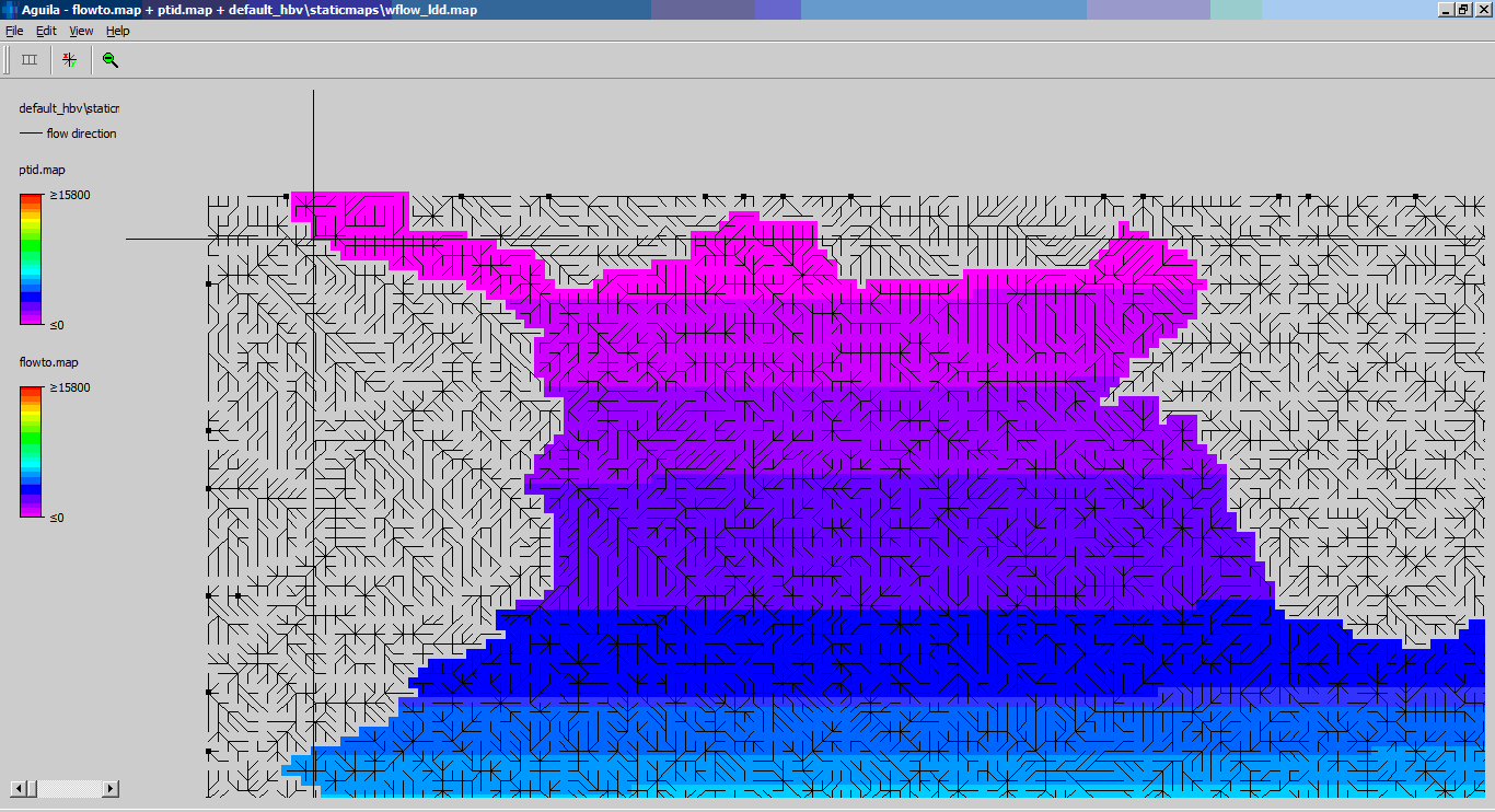
1. The wflow_ldd.map files is used to create the internal flow network, it defines the segments and how water flows between the segments

2. The number of inflows into each segment determines is taken from the sources mapstacks (-S option). Together these sources should include all the water that enters the kinematic wave reservoir. These are the red and green arrows in the figure below

3. The delwaq network is generated for the area define in the wflow_catchment map. The included area is define by all cells were the catchment id in a cel is larger than 1.

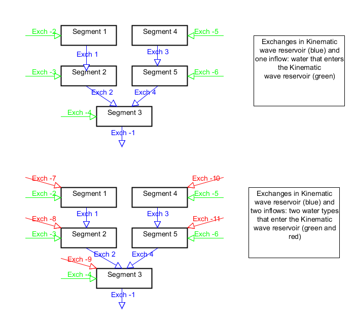
Figure: How exchanges and inflows are connected

Within the includes_flow directory the following files are made:

• volume.dat - volumes (N+1) noseg

• flow.dat - flows (N). Contents is noq

• area.dat - N timesteps. Content is noq

• surface.dat - surface area of the water per segment (N+1), noseq

• length.dat - One timestep only (constant). Content is two times noq

Here nrseg is the number of segments (taken from the non-missing grid cell in the wflow_ldd.map file) and noq is the number of exchanges which is calculated as the number of segments plus number the of inflows (in each segment) times the number of segments

Delwaq expects volumes to be instantanious values at the start of a timestes while flows are integrated between tow timesteps. For volumes N+1 timesteps are needed, for flows N timesteps. The figure below demonstrates this principle for N=4.

The volume.dat file is filled with N+1 steps of volumes of the wflow kinematic wave reservoir. To obtain the needed lag between the flows and the volumes the volumes are taken from the kinematic wave reservoir one timestep back (OldKinWaveVolume).

The flow.dat files is filled as follows. For each timestep internal flows (within the kinematic wave reservoir, i.e. flows from segment to segment) are written first (blue in the layout above). Next the flow into each segment are written. Depending on how many inflow types are given to the script (sources). For one type, one set of flows is written, if there are two types two sets etc (green and red in the layout above).

Very simple example:

The following very simple example demonstrated how the pointer file is created. First the pcraster ldd:

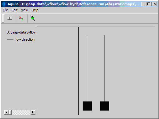
The resulting network consist of 10 points:

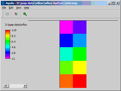
As can be seen both 9 and 10 are bottom points. The generated pointer file is shown below:

 ;Written by dw_WritePointer
 ;nr of pointers is:  20
  1          3          0          0
  2          4          0          0
  3          5          0          0
  4          6          0          0
  5          7          0          0
  6          8          0          0
  7          9          0          0
  8         10          0          0
  9         -1          0          0
 10         -2          0          0
 -3          1          0          0
 -4          2          0          0
 -5          3          0          0
 -6          4          0          0
 -7          5          0          0
 -8          6          0          0
 -9          7          0          0
-10          8          0          0
-11          9          0          0
-12         10          0          0

Case study for Malaysia and Singapore

To estimate load of different nutrients to Johor strait two wflow_sbm models have been setup. Next these models where linked to delwaq as follows:

1. A delwaq segment network similar to the wflow D8 ldd was made

2. The volumes in the delwaq segment are taken from the wflow_sbm kinematic wave volumes

3. For each segment two sources (inflows) are constructed, fast and slow each representing different runoff compartments from the wflow model. Fast represents SOF [1], HOF [2] and SSSF [3] while Slow represent groundwater flow.

4. Next the flow types are combined with the available land-use classes. As such a Luclass times flowtypes matrix of constituents is made. Each constituent (e.g. Slow flow of LU class 1) is traced throughout the system. All constituents are conservative and have a concentration of 1 as they flow in each segement.

5. To check for consistency an Initial water type and a Check water type are introduced. The Initial water will leave the system gradually after a cold start, the Check water type is added to each flow component and should be 1 at each location in the system (Mass Balance Check).

[1]

SOF: Saturation Overland Flow

[2]

HOF: Hortonian Overland Flow (or infiltration excess Overland Flow)

[3]

SSSF: SubSurface Storm Flow. Rapid lateral flow through the top part of the soil profile.

The above results in a system in which the different flow types (including the LU type where they have been generated) can be traced throughout the system. Each each gauge location the discharge and the flow components that make up the discharge are reported.

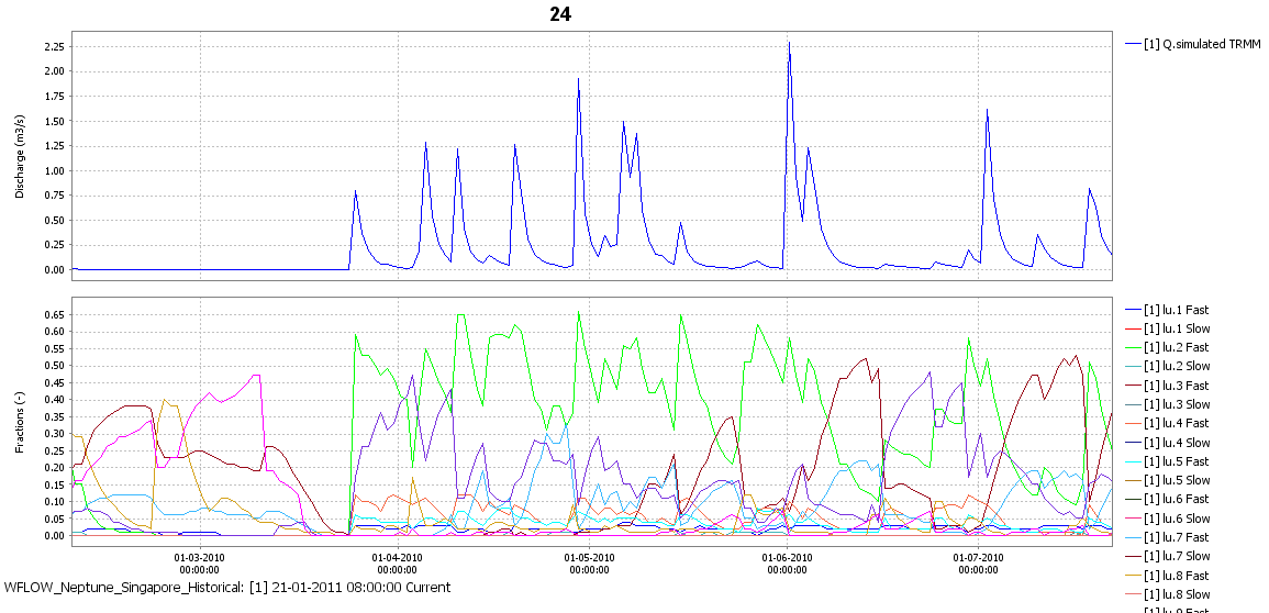
Figure: Discharge and flow types for a small Singapore catchment. The Singapore catchment are dominated by fast flow types but during the end of the dry periods the slow flow types start to rise in importance.

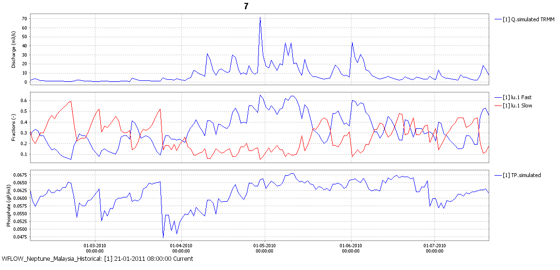
Figure: Discharge, flow types and resulting total P for a catchment in Malaysia.

By assuming each flow type is an end-member in a mixing model we can add fixed concentration of real parameters to the flow fractions and multiply those with the concentrations of the end-membesrt modelled concentration at the gauge locations can be obtained for each timestep.

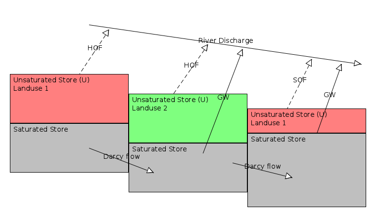
Figure: Flow types in the topog_sbm models used in the Singapore/Malaysia case. HOF = Hortonian or Infiltration excess overland flow. SOF = Saturation overland flow, GW = exfiltrating groundwater. Note that the subcell representation of saturated areas means that both SOF and GW can occur before a cell is completely saturated.

The figure above shows the flow types in the models used in Singapore and Malaysia. Groundwater flow (both from completely saturated cell and subcell groundwater flow) makes up the Slow flow that is fed into the delwaq model while SOF and HOF make up the Fast flow to the delwaq model. In addition the water is also labelled according to the landuse type of the cell that it flows out off.

The whole procedure was setup in a Delft-FEWS configuration that can run the following steps operationally:

wflow_delwaq module documentation