wflow_funcs Module¶

Introduction¶

wflow_funcs is a library of hydrological modules that can be used by any of the wflow models. It includes modules related to:

the kinematic wave routing for surface and subsurface flow
rainfall interception by the vegetation
snow and glaciers modelling
reservoirs and lakes modelling.

Kinematic Wave¶

Surface flow routing¶

The main flow routing scheme used by the wflow models (wflow_sbm and wflow_hbv) is the kinematic wave approach for channel and overland flow, assuming that the topography controls water flow mostly. The kinemative wave equations are (Chow, 1988): $\dfrac{dQ}{dx} + \dfrac{dA}{dt} = q$ and $A = \alpha * Q^{\beta}$. These equations can then be combined as a function of streamflow only:

\[\dfrac{dQ}{dx} + \alpha * \beta * Q^{\beta - 1} * \dfrac{dQ}{dt} = q\]

where $Q$ is the surface runoff in the kinematic wave [m$^{3}$/s], $x$ is the length of the runoff pathway [m], $A$ is the cross-section area of the runoff pathway [m$^{2}$], $t$ is the integration timestep [s] and alpha and beta are coefficients.

These equations are solved with a nonlinear scheme using Newton’s method and can also be iterated depending on the wflow models space and time resolutions. By default, the iterations are performed until a stable solution is reached (epsilon < 10$^{-12}$). For larger models, the number of iterations can also be fixed for wflow_sbm to a specific sub-timestep (in seconds) for both overland and channel flows to improve simulation time. To enable (fixed or not) iterations of the kinematic wave the following lines can be inserted in the ini files of the related models:

[model]
# Enable iterations of the kinematic wave
kinwaveIters = 1
# Fixed sub-timestep for iterations of channel flow (river cells)
kinwaveRiverTstep = 900
# Fixed sub-timestep for iterations of overland flow (land cells)
kinwaveLandTstep = 3600

For wflow_sbm and wflow_hbv Manning’s N values for the river can be specified through a N_River.tbl file in two ways:

N values are linked to land cover (col 1), sub catchment (col 2) and soil type (col 3) (default (NRiverMethod == 1))
N values are linked to streamorder (col 1) (NRiverMethod == 2)

To link N values to streamorder insert the following in the ini file:

[model]
nrivermethod = 2

Subsurface flow routing¶

In wflow_sbm the kinematic wave approach is used to route subsurface flow laterally. The saturated store $S$ can be drained laterally by saturated downslope subsurface flow per unit width of slope $w$ [mm] according to:

\[q=\frac{K_{0}\mathit{tan(\beta)}}{f}(e^{(-fz_{i})}-e^{(-fz_{t})})\]

where $\beta$ is element slope angle [deg.], $q$ is subsurface flow [$mm^{2}/t$], $K_{0}$ is the saturated hydraulic conductivity at the soil surface [mm/t], $z_{i}$ is the water table depth [mm], $z_{t}$ is total soil depth [mm], and $f$ is a scaling parameter [$mm^{-1}$]:

\[f=\frac{\theta_{s}-\theta_{r}}{M}\]

where $\theta_{s}$ is saturated water content [mm/mm] and $\theta_{r}$ is residual water content [mm/mm] and $M$ represents a model parameter [mm], that determines the decrease of vertical saturated conductivity with depth.

Combining with the following continuity equation:

\[(\theta_s-\theta_r)\frac{\partial h}{\partial t} = -w\frac{\partial q}{\partial x} + wr\]

where $h$ is the water table height [mm], $x$ is the distance downslope [mm], and $r$ is the netto input rate [mm/t] to the saturated store.

and substituting for $h (\frac{\partial q}{\partial h})$, gives:

\[w \frac{\partial q}{\partial t} = -cw\frac{\partial q}{\partial x} + cwr\]

where celerity $c = \frac{K_{0}\mathit{tan(\beta)}}{(\theta_s-\theta_r)} e^{(-fz_{i})}$

The kinematic wave equation for lateral subsurface flow is solved iteratively using Newton’s method.

Note

For the lateral subsurface flow kinematic wave the model timestep is not adjusted. For certain model timestep and model grid size combinations this may result in loss of accuracy.

Rainfall Interception¶

Both the Gash and Rutter models are available in the wflow framework to estimate rainfall interception by the vegetation. The selection of an interception model depends on the simulation timestep. These modules are used by the wflow_sbm model.

The analytical (Gash) model¶

The analytical model of rainfall interception is based on Rutter’s numerical model. The simplifications that introduced allow the model to be applied on a daily basis, although a storm-based approach will yield better results in situations with more than one storm per day. The amount of water needed to completely saturate the canopy is defined as:

\[P'=\frac{-\overline{R}S}{\overline{E}_{w}}ln\left[1-\frac{\overline{E}_{w}}{\overline{R}}(1-p-p_{t})^{-1}\right]\]

where $\overline{R}$ is the average precipitation intensity on a saturated canopy and $\overline{E}_{w}$ the average evaporation from the wet canopy and with the vegetation parameters $S$, $p$ and $p_t$ as defined previously. The model uses a series of expressions to calculate the interception loss during different phases of a storm. An analytical integration of the total evaporation and rainfall under saturated canopy conditions is then done for each storm to determine average values of $\overline{E}_{w}$ and $\overline{R}$. The total evaporation from the canopy (the total interception loss) is calculated as the sum of the components listed in the table below. Interception losses from the stems are calculated for days with $P\geq S_{t}/p_{t}$. $p_t$ and $S_t$ are small and neglected in the wflow_sbm model.

Table: Formulation of the components of interception loss according to Gash:

For $m$ small storms ($P_{g}<{P'}_{g}$)	$(1-p-p_{t})\sum_{j=1}^{m}P_{g,j}$
Wetting up the canopy in $n$ large storms ($P_{g}\geq{P'}_{g}$)	$n(1-p-p_{t}){P'}_{g}-nS$
Evaporation from saturated canopy during rainfall	$\overline{E}/\overline{R}\sum_{j=1}^{n}(P_{g,j}-{P'}_{g})$
Evaporation after rainfall ceases for $n$ large storms	$nS$
Evaporation from trunks in $q$ storms that fill the trunk storage	$qS_{t}$
Evaporation from trunks in ($m+n-q$) storms that do not fill the trunk storage	$p_{t}\sum_{j=1}^{m+n-q}P_{g,j}$

In applying the analytical model, saturated conditions are assumed to occur when the hourly rainfall exceeds a certain threshold. Often a threshold of 0.5 mm/hr is used. $\overline{R}$ is calculated for all hours when the rainfall exceeds the threshold to give an estimate of the mean rainfall rate onto a saturated canopy.

Gash (1979) has shown that in a regression of interception loss on rainfall (on a storm basis) the regression coefficient should equal to $\overline{E}_w/\overline{R}$. Assuming that neither $\overline{E}_w$ nor $\overline{R}$ vary considerably in time, $\overline{E}_w$ can be estimated in this way from $\overline{R}$ in the absence of above-canopy climatic observations. Values derived in this way generally tend to be (much) higher than those calculated with the penman-monteith equation.

Running with parameters derived from LAI¶

The model can determine the Gash parameters from an LAI maps. In order to switch this on you must define the LAI variable to the model (as in the example below).

[modelparameters]
LAI=inmaps/clim/LAI,monthlyclim,1.0,1
Sl=inmaps/clim/LCtoSpecificLeafStorage.tbl,tbl,0.5,1,inmaps/clim/LC.map
Kext=inmaps/clim/LCtoExtinctionCoefficient.tbl,tbl,0.5,1,inmaps/clim/LC.map
Swood=inmaps/clim/LCtoBranchTrunkStorage.tbl,tbl,0.5,1,inmaps/clim/LC.map

Here LAI refers to a MAP with LAI (in this case one per month), Sl to a lookuptable result of land cover to specific leaf storage, Kext to a lookuptable result of land cover to extinction coefficient and Swood to a lookuptable result of “canopy” capacity of the vegetation woody fraction.

Here it is assumed that Cmax(leaves) (Gash’ canopy capacity for the leaves only) relates linearly with LAI (c.f. Van Dijk and Bruijnzeel 2001). This done via the Sl (specific leaf storage). Sl is determined via a lookup table with land cover. Next the Cmax(leaves) is determined using:

\[Cmax(leaves) = Sl * LAI\]

The table below shows lookup table for Sl (as determined from Pitman 1986, Lui 1998) and GlobCover land cover map.

 0.1272    Post-flooding or irrigated croplands (or aquatic)
 0.1272    Rainfed croplands
 0.1272    Mosaic cropland (50-70%) / vegetation (grassland/shrubland/forest) (20-50%)
 0.1272    Mosaic vegetation (grassland/shrubland/forest) (50-70%) / cropland (20-50%)
 0.03926   Closed to open (>15%) broadleaved evergreen or semi-deciduous forest (>5m)
 0.036     Closed (>40%) broadleaved deciduous forest (>5m)
 0.036     Open (15-40%) broadleaved deciduous forest/woodland (>5m)
 0.045     Closed (>40%) needleleaved evergreen forest (>5m)
 0.045     Open (15-40%) needleleaved deciduous or evergreen forest (>5m)
0.03926   Closed to open (>15%) mixed broadleaved and needleleaved forest (>5m)
0.07      Mosaic forest or shrubland (50-70%) / grassland (20-50%)
0.1272    Mosaic grassland (50-70%) / forest or shrubland (20-50%)
0.07      Closed to open (>15%) (broadleaved or needleleaved, evergreen or deciduous) shrubland (<5m)
0.09      Closed to open (>15%) herbaceous vegetation (grassland, savannas or lichens/mosses)
0.04      Sparse (<15%) vegetation
0.04      Closed to open (>15%) broadleaved forest regularly flooded (semi-permanently or temporarily) - Fresh or brackish water
0.036     Closed (>40%) broadleaved forest or shrubland permanently flooded - Saline or brackish water
0.1272    Closed to open (>15%) grassland or woody vegetation on regularly flooded or waterlogged soil - Fresh, brackish or saline water
0.04      Artificial surfaces and associated areas (Urban areas >50%)
0.04      Bare areas
0.04      Water bodies
0.04      Permanent snow and ice
 -        No data (burnt areas, clouds,…)

To get to total storage (Cmax) the woody part of the vegetation also needs to be added. This is done via a simple lookup table between land cover the Cmax(wood):

digraph cmax {
"GlobCover LandCover" -> "Sl lookuptable";
"Sl lookuptable" -> Sl -> Multiply;
"LAI (monthly)" -> Multiply -> "Cmax (leaves)" -> add;
"GlobCover LandCover" -> "Cmax Wood lookuptable";
"Cmax Wood lookuptable" -> "Cmax (wood)";
"Cmax (wood)"-> add;
add -> Cmax;
}

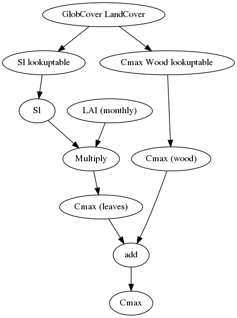
The table below relates the land cover map to the woody part of the Cmax.

 0.01    Post-flooding or irrigated croplands (or aquatic)
 0.0     Rainfed croplands
 0.01    Mosaic cropland (50-70%) / vegetation (grassland/shrubland/forest) (20-50%)
 0.01    Mosaic vegetation (grassland/shrubland/forest) (50-70%) / cropland (20-50%)
 0.5     Closed to open (>15%) broadleaved evergreen or semi-deciduous forest (>5m)
 0.5     Closed (>40%) broadleaved deciduous forest (>5m)
 0.5     Open (15-40%) broadleaved deciduous forest/woodland (>5m)
 0.5     Closed (>40%) needleleaved evergreen forest (>5m)
 0.5     Open (15-40%) needleleaved deciduous or evergreen forest (>5m)
0.5     Closed to open (>15%) mixed broadleaved and needleleaved forest (>5m)
0.2     Mosaic forest or shrubland (50-70%) / grassland (20-50%)
0.05    Mosaic grassland (50-70%) / forest or shrubland (20-50%)
0.1     Closed to open (>15%) (broadleaved or needleleaved, evergreen or deciduous) shrubland (<5m)
0.0     Closed to open (>15%) herbaceous vegetation (grassland, savannas or lichens/mosses)
0.04    Sparse (<15%) vegetation
0.1     Closed to open (>15%) broadleaved forest regularly flooded (semi-permanently or temporarily) - Fresh or brackish water
0.2     Closed (>40%) broadleaved forest or shrubland permanently flooded - Saline or brackish water
0.01    Closed to open (>15%) grassland or woody vegetation on regularly flooded or waterlogged soil - Fresh, brackish or saline water
0.01    Artificial surfaces and associated areas (Urban areas >50%)
0.0     Bare areas
0.0     Water bodies
0.0     Permanent snow and ice
 -      No data (burnt areas, clouds,…)

The canopy gap fraction is determined using the k: extinction coefficient (van Dijk and Bruijnzeel 2001):

\[CanopyGapFraction = exp(-k * LAI)\]

The table below show how k is related to land cover:

 0.6    Post-flooding or irrigated croplands (or aquatic)
 0.6    Rainfed croplands
 0.6    Mosaic cropland (50-70%) / vegetation (grassland/shrubland/forest) (20-50%)
 0.6    Mosaic vegetation (grassland/shrubland/forest) (50-70%) / cropland (20-50%)
 0.6    Closed to open (>15%) broadleaved evergreen or semi-deciduous forest (>5m)
 0.8    Closed (>40%) broadleaved deciduous forest (>5m)
 0.8    Open (15-40%) broadleaved deciduous forest/woodland (>5m)
 0.8    Closed (>40%) needleleaved evergreen forest (>5m)
 0.8    Open (15-40%) needleleaved deciduous or evergreen forest (>5m)
0.8    Closed to open (>15%) mixed broadleaved and needleleaved forest (>5m)
0.6    Mosaic forest or shrubland (50-70%) / grassland (20-50%)
0.6    Mosaic grassland (50-70%) / forest or shrubland (20-50%)
0.6    Closed to open (>15%) (broadleaved or needleleaved, evergreen or deciduous) shrubland (<5m)
0.6    Closed to open (>15%) herbaceous vegetation (grassland, savannas or lichens/mosses)
0.6    Sparse (<15%) vegetation
0.6    Closed to open (>15%) broadleaved forest regularly flooded (semi-permanently or temporarily) - Fresh or brackish water
0.8    Closed (>40%) broadleaved forest or shrubland permanently flooded - Saline or brackish water
0.6    Closed to open (>15%) grassland or woody vegetation on regularly flooded or waterlogged soil - Fresh, brackish or saline water
0.6    Artificial surfaces and associated areas (Urban areas >50%)
0.6    Bare areas
0.7    Water bodies
0.6    Permanent snow and ice
 -     No data (burnt areas, clouds,…)d

The modified rutter model¶

For subdaily timesteps the model uses a simplification of the Rutter model. The simplified model is solved explicitly and does not take drainage from the canopy into account.

def rainfall_interception_modrut(Precipitation, PotEvap, CanopyStorage, CanopyGapFraction, Cmax):
"""
Interception according to a modified Rutter model. The model is solved
explicitly and there is no drainage below Cmax.

Returns:
    - NetInterception: P - TF - SF (may be different from the actual wet canopy evaporation)
    - ThroughFall:
    - StemFlow:
    - LeftOver: Amount of potential eveporation not used
    - Interception: Actual wet canopy evaporation in this thimestep
    - CanopyStorage: Canopy storage at the end of the timestep

"""

##########################################################################
# Interception according to a modified Rutter model with hourly timesteps#
##########################################################################

p = CanopyGapFraction
pt = 0.1 * p

# Amount of P that falls on the canopy
Pfrac = pcr.max((1 - p - pt), 0) * Precipitation

# S cannot be larger than Cmax, no gravity drainage below that
DD = pcr.ifthenelse(CanopyStorage > Cmax, CanopyStorage - Cmax, 0.0)
CanopyStorage = CanopyStorage - DD

# Add the precipitation that falls on the canopy to the store
CanopyStorage = CanopyStorage + Pfrac

# Now do the Evap, make sure the store does not get negative
dC = -1 * pcr.min(CanopyStorage, PotEvap)
CanopyStorage = CanopyStorage + dC

LeftOver = PotEvap + dC
# Amount of evap not used

# Now drain the canopy storage again if needed...
D = pcr.ifthenelse(CanopyStorage > Cmax, CanopyStorage - Cmax, 0.0)
CanopyStorage = CanopyStorage - D

# Calculate throughfall
ThroughFall = DD + D + p * Precipitation
StemFlow = Precipitation * pt

# Calculate interception, this is NET Interception
NetInterception = Precipitation - ThroughFall - StemFlow
Interception = -dC

return NetInterception, ThroughFall, StemFlow, LeftOver, Interception, CanopyStorage

Snow and Glaciers¶

Snow and glaciers processes, from the HBV model, are available in the wflow framework. The snow and glacier functions are used by the wflow_sbm model, and the glacier function is used by the wflow_hbv model.

Snow modelling¶

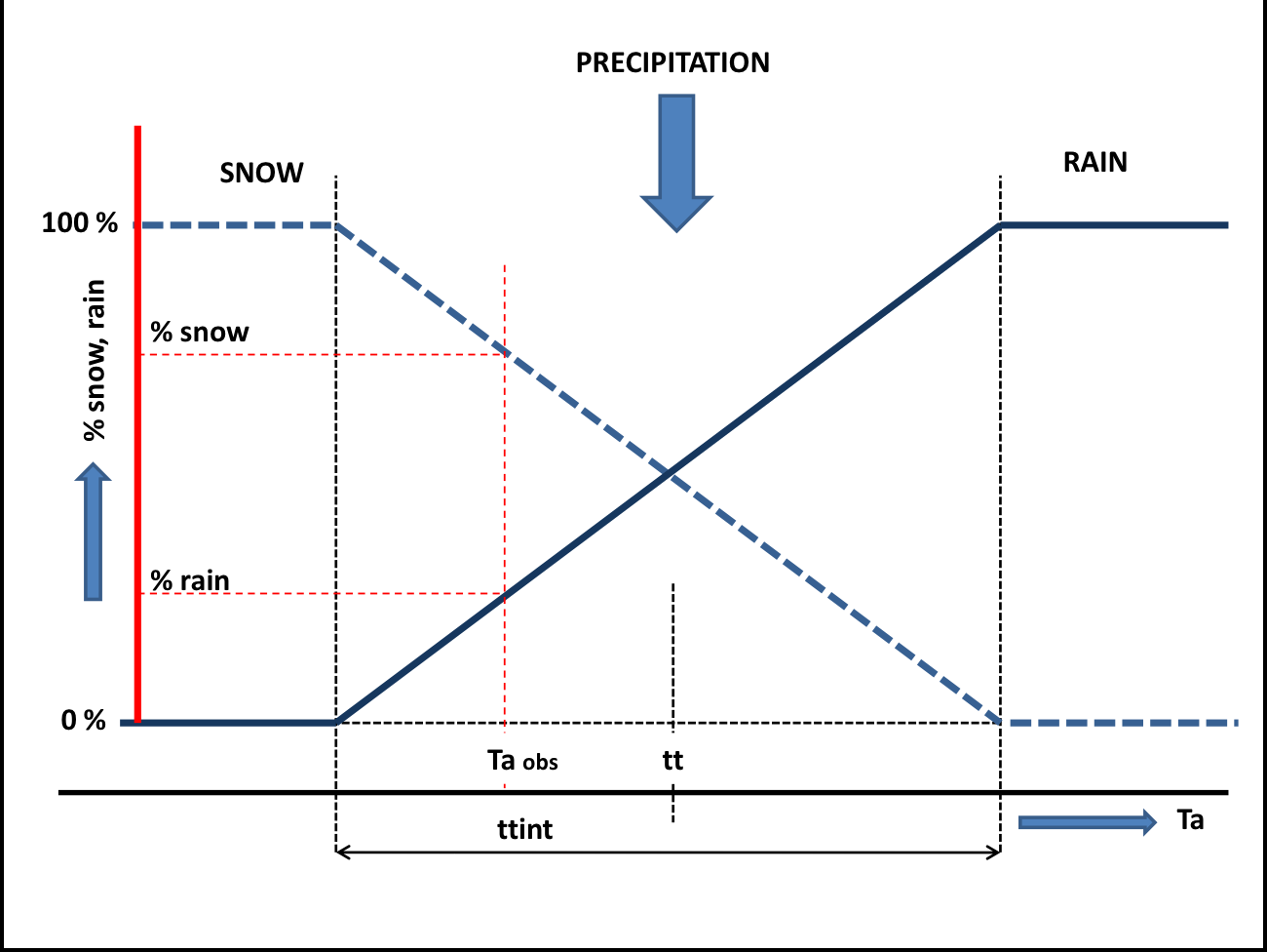
If the air temperature, $T_{a}$, is below a user-defined threshold $TT (\approx0^{o}C)$ precipitation occurs as snowfall, whereas it occurs as rainfall if $T_{a}\geq TT$. A another parameter $TTI$ defines how precipitation can occur partly as rain of snowfall (see the figure below). If precipitation occurs as snowfall, it is added to the dry snow component within the snow pack. Otherwise it ends up in the free water reservoir, which represents the liquid water content of the snow pack. Between the two components of the snow pack, interactions take place, either through snow melt (if temperatures are above a threshold $TT$) or through snow refreezing (if temperatures are below threshold $TT$). The respective rates of snow melt and refreezing are:

\[ \begin{align}\begin{aligned}Q_{m} = cfmax(T_{a}-TT)\;\;;T_{a}>TT\\Q_{r} = cfmax*cfr(TT-T_{a})\;;T_{a}<TT\end{aligned}\end{align} \]

where $Q_{m}$ is the rate of snow melt, $Q_{r}$ is the rate of snow refreezing, and $cfmax$ and $cfr$ are user defined model parameters (the melting factor $mm/(^{o}C*day)$ and the refreezing factor respectively)

Note

The FoCFMAX parameter from the original HBV version is not used. instead the CFMAX is presumed to be for the landuse per pixel. Normally for forested pixels the CFMAX is 0.6 {*} CFMAX

The air temperature, $T_{a}$, is related to measured daily average temperatures. In the original HBV-concept, elevation differences within the catchment are represented through a distribution function (i.e. a hypsographic curve) which makes the snow module semi-distributed. In the modified version that is applied here, the temperature, $T_{a}$, is represented in a fully distributed manner, which means for each grid cell the temperature is related to the grid elevation.

The fraction of liquid water in the snow pack (free water) is at most equal to a user defined fraction, $WHC$, of the water equivalent of the dry snow content. If the liquid water concentration exceeds $WHC$, either through snow melt or incoming rainfall, the surpluss water becomes available for infiltration into the soil:

\[Q_{in}=max\{(SW-WHC*SD);\;0.0\}\]

where $Q_{in}$ is the volume of water added to the soil module, $SW$ is the free water content of the snow pack and $SD$ is the dry snow content of the snow pack.

Schematic view of the snow routine¶

Glacier modelling¶

Glacier processes can be modelled if the snow model is enabled in wflow_sbm. For wflow_hbv snow modelling is not optional. Glacier modelling is very close to snow modelling and considers two main processes: glacier build-up from snow turning into firn/ice (using the HBV-light model) and glacier melt (using a temperature degree-day model).

The definition of glacier boundaries and initial volume is defined in three staticmaps. GlacierAreas is a map containing the ID of the glacier present in the wflow cell. GlacierFrac is a map that gives the fraction of each grid cell covered by a glacier as a number between zero and one. GlacierStore is a state map that gives the amount of water (in mm w.e.) within the glaciers at each gridcell. Because the glacier store (GlacierStore.map) cannot be initialized by running the model for a couple of years, a default initial state map should be supplied by placing a GlacierStore.map file in the staticmaps directory. These three maps are prepared from available glacier datasets.

First, a fixed fraction of the snowpack on top of the glacier is converted into ice for each timestep and added to the glacier store using the HBV-light model (Seibert et al.,2017). This fraction, defined in the lookup table G_SIfrac, typically ranges from 0.001 to 0.006.

Then, when the snowpack on top of the glacier is almost all melted (snow cover < 10 mm), glacier melt is enabled and estimated with a degree-day model. If the air temperature, $T_{a}$, is below a certain threshold $G\_TT (\approx0^{o}C)$ precipitation occurs as snowfall, whereas it occurs as rainfall if $T_{a}\geq G\_TT$.

With this the rate of glacier melt in mm is estimated as:

\[Q_{m} = G\_Cfmax(T_{a}-G\_TT)\;\;;T_{a}>G\_TT\]

where $Q_{m}$ is the rate of glacier melt and $G\_Cfmax$ is the melting factor in $mm/(^{o}C*day)$. Parameters G_TT and G_Cfmax are defined in two lookup tables. G_TT can be taken as equal to the snow TT parameter. Values of the melting factor normally varies from one glacier to another and some values are reported in the literature. G_Cfmax can also be estimated by multiplying snow Cfmax by a factor between 1 and 2, to take into account the higher albedo of ice compared to snow.

Glacier modelling can be enabled by including the following four entries in the modelparameters section:

[modelparameters]
GlacierAreas = staticmaps/wflow_glacierareas.map,staticmap,0.0,0
GlacierFrac = staticmaps/wflow_glacierfrac.map,staticmap,0.0,0
G_TT = intbl/G_TT.tbl,tbl,0.0,1,staticmaps/wflow_glacierareas.map
G_Cfmax = intbl/G_Cfmax.tbl,tbl,3.0,1,staticmaps/wflow_glacierareas.map
G_SIfrac = intbl/G_SIfrac.tbl,tbl,0.001,1,staticmaps/wflow_glacierareas.map

The initial glacier volume wflow_glacierstore.map should also be added in the staticmaps folder.

Reservoirs and Lakes¶

Simplified reservoirs and lakes models are included in the framwork and used by the wflow_sbm, wflow_hbv and wflow_routing models.

Reservoirs¶

Simple reservoirs can be included within the kinematic wave routing by supplying two maps, one map with the outlet of the reservoirs in which each reservoir has a unique id (ReserVoirSimpleLocs), and one map with the extent of reservoir (ReservoirSimpleAreas). Furthermore a set of lookuptables must be defined linking the reservoir-id’s to reservoir characteristics:

ResTargetFullFrac.tbl - Target fraction full (of max storage) for the reservoir: number between 0 and 1
ResTargetMinFrac.tbl - Target minimum full fraction (of max storage). Number between 0 and 1 < ResTargetFullFrac
ResMaxVolume.tbl - Maximum reservoir storage (above which water is spilled) [m$^3$]
ResDemand.tbl - Minimum (environmental) flow requirement downstream of the reservoir m$^3$/s
ResMaxRelease.tbl - Maximum Q that can be released if below spillway [m$^3$/s]
ResSimpleArea.tbl - Surface area of the reservoir [m$^{2}$]

By default the reservoirs are not included in the model. To include them put the following lines in the .ini file of the model.

[modelparameters]
# Add this if you want to model reservoirs
ReserVoirSimpleLocs=staticmaps/wflow_reservoirlocs.map,staticmap,0.0,0
ReservoirSimpleAreas=staticmaps/wflow_reservoirareas.map,staticmap,0.0,0
ResSimpleArea = intbl/ResSimpleArea.tbl,tbl,0,0,staticmaps/wflow_reservoirlocs.map
ResTargetFullFrac=intbl/ResTargetFullFrac.tbl,tbl,0.8,0,staticmaps/wflow_reservoirlocs.map
ResTargetMinFrac=intbl/ResTargetMinFrac.tbl,tbl,0.4,0,staticmaps/wflow_reservoirlocs.map
ResMaxVolume=intbl/ResMaxVolume.tbl,tbl,0.0,0,staticmaps/wflow_reservoirlocs.map
ResMaxRelease=intbl/ResMaxRelease.tbl,tbl,1.0,0,staticmaps/wflow_reservoirlocs.map
ResDemand=intbl/ResDemand.tbl,tblmonthlyclim,1.0,0,staticmaps/wflow_reservoirlocs.map

In the above example most values are fixed thoughout the year, only the ResDemand is in given per month of the year.

Natural Lakes¶

Natural (uncontrolled) lakes can be modelled in wflow using a mass balance approach:

\[\dfrac{S(t + \Delta t)}{\Delta t} = \dfrac{S(t)}{\Delta t} + Q_{in} + \dfrac{(P-E)*A}{\Delta t} - Q_{out}\]

where $S$ is lake storage [m$^{3}$], $\Delta t$ is the model timestep [seconds], $Q_{in}$ is the sum of inflows (surface runoff and seepage) [m$^{3}$/s], $Q_{out}$ is the lake outflow at the outlet [m$^{3}$/s], $P$ is precipitation [m], $E$ is lake evaporation [m] and $A$ is lake surface.

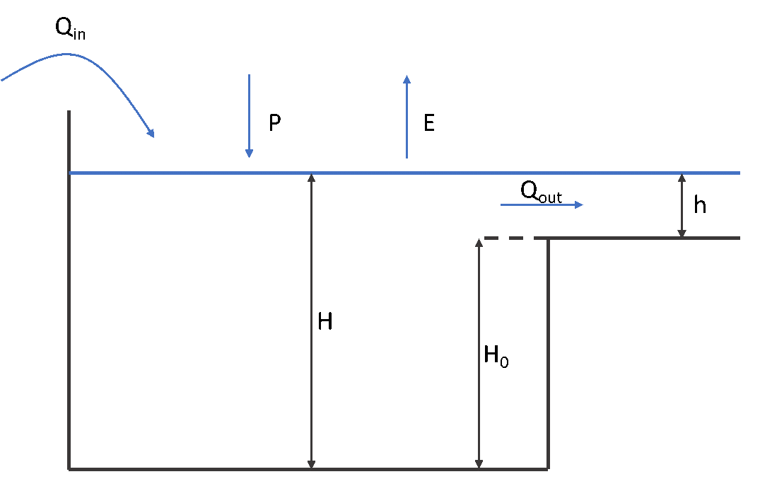
Lake schematisation.¶

Most of the variables in this equation are already known or coming from previous timestep, apart from $S(t+ \Delta t)$ and $Q_{out}$ which can both be linked to the water level $H$ in the lake using a storage curve $S = f(H)$ and a rating curve $Q = f(H)$. In wflow, several options are available to select storage and rating curves, and in most cases, the mass balance is then solved by linearization and iteration or using the Modified Puls Approach from Maniak (Burek et al., 2013). Storage curves in wflow can either:

Come from the interpolation of field data linking volume and lake height,
Be computed from the simple relationship $S = A*H$.

Rating curves in wlow can either:

Come from the interpolation of field data linking lake outflow and water height,
Be computed from a rating curve of the form $Q_{out} = \alpha *{(H-H_{0})}^{\beta}$, where $H_{0}$ is the minimum water level under which the outflow is zero. Usual values for $\beta$ are 3/2 for a rectangular weir or 2 for a parabolic weir (Bos, 1989).

Modified Puls Approach¶

The Modified Puls Approach is a resolution method of the lake balance that uses an explicit relationship between storage and outflow. Storage is assumed to be equal to A*H and the rating curve for a parabolic weir (beta =2):

\[S = A*H = A * (h + H_{0}) = \dfrac{A}{\sqrt{\alpha}} \sqrt{Q} + A*H_{0}\]

Inserting this equation in the mass balance gives:

\[\dfrac{A}{\Delta t \sqrt{\alpha}} \sqrt{Q} + Q = \dfrac{S(t)}{\Delta t} + Q_{in} + \dfrac{(P-E)*A}{\Delta t} - \dfrac{A*H_{0}}{\Delta t} = SI - \dfrac{A*H_{0}}{\Delta t}\]

The solution for Q is then:

$Q = { \left( -LF + \sqrt{LF^{2} + 2 * \left( SI - \dfrac{A*H_{0}}{\Delta t} \right) } \right) }^{2}$ for $SI > \dfrac{A*H_{0}}{\Delta t}$ and where $LF = \dfrac{A}{\Delta t \sqrt{\alpha}}$
$Q = 0$ for $SI \leq \dfrac{A*H_{0}}{\Delta t}$

Setup and input files¶

Natural lakes can be included within the kinematic wave routing in wflow, by supplying two maps with the locations of the lakes (one map for the extents, LakeAreas.map, and one for the outlets, LakeLocs.map) and in which each lake has a unique id. Furthermore a set of lookuptables must be deﬁned linking the lake id’s to lake characteristics:

LakeArea: surface area of the lakes [m$^{2}$]
LakeAvgLevel: average lake water level [m], used to reinitiate model states [m].
LakeThreshold: water level threshold H$_{0}$ under which outflow is zero [m].
LakeStorFunc: type of lake storage curve ; 1 for S = AH (default) and 2 for S = f(H) from lake data and interpolation.
LakeOutflowFunc: type of lake rating curve ; 1 for Q = f(H) from lake data and interpolation, 2 for general Q = b(H - H$_{0}$)$^{e}$ and 3 in the case of Puls Approach Q = b(H - H$_{0}$)$^{2}$ (default).
Lake_b: rating curve coefficient.
Lake_e: rating curve exponent.

By default, the lakes are not included in the model. To include them, put the following lines in the .ini ﬁle of the model:

LakeLocs=staticmaps/wflow_lakelocs.map,staticmap,0.0,0
LakeAreasMap=staticmaps/wflow_lakeareas.map,staticmap,0.0,0
LinkedLakeLocs=intbl/LinkedLakeLocs.tbl,tbl,0,0,staticmaps/wflow_lakelocs.map
LakeStorFunc = intbl/LakeStorFunc.tbl,tbl,1,0,staticmaps/wflow_lakelocs.map
LakeOutflowFunc = intbl/LakeOutflowFunc.tbl,tbl,3,0,staticmaps/wflow_lakelocs.map
LakeArea = intbl/LakeArea.tbl,tbl,1,0,staticmaps/wflow_lakelocs.map
LakeAvgLevel = intbl/LakeAvgLevel.tbl,tbl,1,0,staticmaps/wflow_lakelocs.map
LakeAvgOut = intbl/LakeAvgOut.tbl,tbl,1,0,staticmaps/wflow_lakelocs.map
LakeThreshold = intbl/LakeThreshold.tbl,tbl,0,0,staticmaps/wflow_lakelocs.map
Lake_b = intbl/Lake_b.tbl,tbl,50,0,staticmaps/wflow_lakelocs.map
Lake_e = intbl/Lake_e.tbl,tbl,2.0,0,staticmaps/wflow_lakelocs.map

Additional settings¶

Storage / rating curve from data

Storage and rating curves coming from field measurement can be supplied to wflow via tbl files supplied in the intbl folder. Naming of the files uses the ID of the lakes where data are available and is of the form Lake_SH_1.tbl and Lake_HQ_1.tbl for respectively the storage and rating curves of lake with ID 1.

The storage curve is a tbl with lake level [m] in the first column and corresponding lake storage [m$^{3}$] in the second column.

The rating curve uses level and discharge data depending on the Julian day of the year (JDOY). The first line contains the minimum level and corresponding average yearly discharge, and the second line the maximum level and corresponding average yearly discharge. The third line contains first a blank cell and numbers for the days of the year (from 1 to 365). The other lines contain the water level and the corresponding discharges for the different JDOY (example below).

00   43.000
00 1260.000
                 1          2           3 …       364         365
00      43.000     43.000      43.000 …    43.000      43.000
01      44.838     44.838      44.838 …    44.838      44.838
…
99 1256.229 1256.229 1256.229 … 1256.229 1256.229
00 1260.000 1260.000 1260.000 … 1260.000 1260.000

Estimating the lake water level threshold for outflow

By default, the lake water level threshold (for which lake ouflow is zero) is set to zero. For some more specific studies, this threshold can be estimated using the lake average outflow and level as well as the river characteristics at the outlet (relationship between discharge and water level from the kinematic wave). After estimation of the threshold, the parameter $\alpha$ from the lake rating curve is also adjusted.

To enable this option, the line estimatelakethresh = 1 should be added to the [model] section of the ini file (default value is 0), and the tbls LakeAvgOut [m$^{3}$/s] and LakeAvgLevel [m] with the lake average ouflow and level should be supplied.

Linked lakes

In some cases, close lakes can be linked and return flow can be allowed from the downstream to the upstream lake. The linked lakes are defined in the LinkedLakeLocs.tbl file by linking the lake ID of the upstream lake (first column) to the ID of the linked downstream lake (second column).

Note: in every file, level units are meters [m] and NOT meters above sea level [m asl]. Especially with storage/rating curves coming from data, please be careful and convert units if needed.

References¶

Burek P., Van der Knijf J.M., Ad de Roo, 2013. LISFLOOD – Distributed Water Balance and flood Simulation Model – Revised User Manual. DOI: http://dx.doi.org/10.2788/24719.
Bos M.G., 1989. Discharge measurement structures. Third revised edition, International Institute for Land Reclamation and Improvement ILRI, Wageningen, The Netherlands.

wflow_funcs module documentation¶

wflow_funcs - hydrological functions library¶

In addition this library contain a number of hydrological functions that may be used within the wflow models

It contains both the kinematic wave, interception, snow/glaciers and reservoirs/lakes modules.

wflow_funcs.SnowPackHBV(Snow, SnowWater, Precipitation, Temperature, TTI, TT, TTM, Cfmax, WHC)¶

HBV Type snowpack modelling using a Temperature degree factor. All correction factors (RFCF and SFCF) are set to 1. The refreezing efficiency factor is set to 0.05.

Parameters

Snow –
SnowWater –
Precipitation –
Temperature –
TTI –
TT –
TTM –
Cfmax –
WHC –

Returns

Snow,SnowMelt,Precipitation

wflow_funcs.bf_oneparam(discharge, k)¶

wflow_funcs.bf_threeparam(discharge, k, C, a)¶

wflow_funcs.bf_twoparam(discharge, k, C)¶

wflow_funcs.estimate_iterations_kin_wave(Q, Beta, alpha, timestepsecs, dx, mv)¶

wflow_funcs.glacierHBV(GlacierFrac, GlacierStore, Snow, Temperature, TT, Cfmax, G_SIfrac, timestepsecs, basetimestep)¶

Run Glacier module and add the snowpack on-top of it. First, a fraction of the snowpack is converted into ice using the HBV-light model (fraction between 0.001-0.005 per day). Glacier melting is modelled using a Temperature degree factor and only occurs if the snow cover < 10 mm.

Variables

GlacierFrac – Fraction of wflow cell covered by glaciers
GlacierStore – Volume of the galcier in the cell in mm w.e.
Snow – Snow pack on top of Glacier
Temperature – Air temperature
TT – Temperature threshold for ice melting
Cfmax – Ice degree-day factor in mm/(°C/day)
G_SIfrac – Fraction of the snow part turned into ice each timestep
timestepsecs – Model timestep in seconds
basetimestep – Model base timestep (86 400 seconds)

Returns

Snow,Snow2Glacier,GlacierStore,GlacierMelt,

wflow_funcs.kin_wave(rnodes, rnodes_up, Qold, q, Alpha, Beta, DCL, River, Bw, AlpTermR, AlpPow, deltaT, it=1)¶

wflow_funcs.kinematic_wave(Qin, Qold, q, alpha, beta, deltaT, deltaX)¶

wflow_funcs.kinematic_wave_ssf(ssf_in, ssf_old, zi_old, r, Ks_hor, Ks, slope, neff, f, D, dt, dx, w, ssf_max)¶

wflow_funcs.lookupResFunc(ReserVoirLocs, values, sh, dirLookup)¶

wflow_funcs.lookupResRegMatr(ReserVoirLocs, values, hq, JDOY)¶

wflow_funcs.naturalLake(waterlevel, LakeLocs, LinkedLakeLocs, LakeArea, LakeThreshold, LakeStorFunc, LakeOutflowFunc, sh, hq, lake_b, lake_e, inflow, precip, pet, LakeAreasMap, JDOY, timestepsecs=86400)¶

Run Natural Lake module to compute the new waterlevel and outflow. Solves lake water balance with linearisation and iteration procedure, for any rating and storage curve. For the case where storage curve is S = AH and Q=b(H-Ho)^2, uses the direct solution from the Modified Puls Approach (LISFLOOD).

Variables

waterlevel – water level H in the lake
LakeLocs – location of lake’s outlet
LinkedLakeLocs – ID of linked lakes
LakeArea – total lake area
LakeThreshold – water level threshold Ho under which outflow is zero
LakeStorFunc – type of lake storage curve 1: S = AH 2: S = f(H) from lake data and interpolation
LakeOutflowFunc – type of lake rating curve 1: Q = f(H) from lake data and interpolation 2: General Q = b(H - Ho)^e 3: Case of Puls Approach Q = b(H - Ho)^2
sh – data for storage curve
hq – data for rating curve
lake_b – rating curve coefficient
lake_e – rating curve exponent
inflow – inflow to the lake (surface runoff + river discharge + seepage)
precip – precipitation map
pet – PET map
LakeAreasMap – lake extent map (for filtering P and PET)
JDOY – Julian Day of Year to read storage/rating curve from data
timestepsecs – model timestep in seconds

Returns

waterlevel, outflow, prec_av, pet_av, storage

wflow_funcs.propagate_downstream(rnodes, rnodes_up, material)¶

wflow_funcs.rainfall_interception_gash(Cmax, EoverR, CanopyGapFraction, Precipitation, CanopyStorage, maxevap=9999)¶: Interception according to the Gash model (For daily timesteps).

wflow_funcs.rainfall_interception_hbv(Rainfall, PotEvaporation, Cmax, InterceptionStorage)¶: Returns: TF, Interception, IntEvap,InterceptionStorage

wflow_funcs.rainfall_interception_modrut(Precipitation, PotEvap, CanopyStorage, CanopyGapFraction, Cmax)¶

Interception according to a modified Rutter model. The model is solved explicitly and there is no drainage below Cmax.

Returns:

NetInterception: P - TF - SF (may be different from the actual wet canopy evaporation)
ThroughFall:
StemFlow:
LeftOver: Amount of potential eveporation not used
Interception: Actual wet canopy evaporation in this thimestep
CanopyStorage: Canopy storage at the end of the timestep

wflow_funcs.sCurve(X, a=0.0, b=1.0, c=1.0)¶

sCurve function:

Input:

X input map
C determines the steepness or “stepwiseness” of the curve. The higher C the sharper the function. A negative C reverses the function.
b determines the amplitude of the curve
a determines the centre level (default = 0)

Output:

result

wflow_funcs.set_dd(ldd, _ldd_us=array([[3, 2, 1], [6, 5, 4], [9, 8, 7]]), pit_value=5)¶: set drainage direction network from downstream to upstream

wflow_funcs.simplereservoir(storage, inflow, ResArea, maxstorage, target_perc_full, maximum_Q, demand, minimum_full_perc, ReserVoirLocs, precip, pet, ReservoirSimpleAreas, timestepsecs=86400)¶

Parameters

storage – initial storage m^3
inflow – inflow m^3/s
maxstorage – maximum storage (above which water is spilled) m^3
target_perc_full – target fraction full (of max storage) -
maximum_Q – maximum Q to release m^3/s if below spillway
demand – water demand (all combined) m^3/s
minimum_full_perc – target minimum full fraction (of max storage) -
ReserVoirLocs – map with reservoir locations
timestepsecs – timestep of the model in seconds (default = 86400)

Returns

storage (m^3), outflow (m^3/s), PercentageFull (0-1), Release (m^3/sec)

For \(m\) small storms (\(P_{g}<{P'}_{g}\))	\((1-p-p_{t})\sum_{j=1}^{m}P_{g,j}\)
Wetting up the canopy in \(n\) large storms (\(P_{g}\geq{P'}_{g}\))	\(n(1-p-p_{t}){P'}_{g}-nS\)
Evaporation from saturated canopy during rainfall	\(\overline{E}/\overline{R}\sum_{j=1}^{n}(P_{g,j}-{P'}_{g})\)
Evaporation after rainfall ceases for \(n\) large storms	\(nS\)
Evaporation from trunks in \(q\) storms that fill the trunk storage	\(qS_{t}\)
Evaporation from trunks in (\(m+n-q\)) storms that do not fill the trunk storage	\(p_{t}\sum_{j=1}^{m+n-q}P_{g,j}\)